# Dot product
> Source: https://aiwiki.ai/wiki/dot_product
> Updated: 2026-11-18
> Fact-checked: 2026-11-18
> Categories: Deep Learning, Machine Learning, Mathematics
> License: CC BY 4.0 (https://creativecommons.org/licenses/by/4.0/) - attribute to "AI Wiki (aiwiki.ai)"
> Cite as: AI Wiki. "Dot product." aiwiki.ai, 18 Nov 2026. https://aiwiki.ai/wiki/dot_product
> From AI Wiki (https://aiwiki.ai), the free encyclopedia of artificial intelligence. Reuse freely with attribution.
The **dot product** (also called the **scalar product**, and in real coordinate space the standard **inner product**) is an operation that takes two vectors of the same length and returns a single number: the sum of the products of their corresponding entries [1]. Geometrically, the same number equals the product of the two vectors' lengths and the cosine of the angle between them, so it measures how far two vectors point in the same direction [2]. The operation grew out of nineteenth-century work on quaternions and vector algebra [3], and its name and dot notation come from the vector analysis that J. Willard Gibbs taught at Yale, as written up by Edwin Bidwell Wilson in 1901 [4]. In [machine learning](https://aiwiki.ai/wiki/machine_learning) it is a basic building block: a typical [neuron](https://aiwiki.ai/wiki/neuron) in a feedforward network computes a dot product between its weights and its inputs [5], [attention](https://aiwiki.ai/wiki/attention) in [transformers](https://aiwiki.ai/wiki/transformers) scores queries against keys with dot products [6], and dense retrieval systems rank documents by the dot product of learned [embeddings](https://aiwiki.ai/wiki/embeddings) [7].
Each entry of a matrix product is itself a dot product [2], and a 2018 paper on mixed-precision training sorted neural network arithmetic into three categories, the first of which is vector dot products [8].
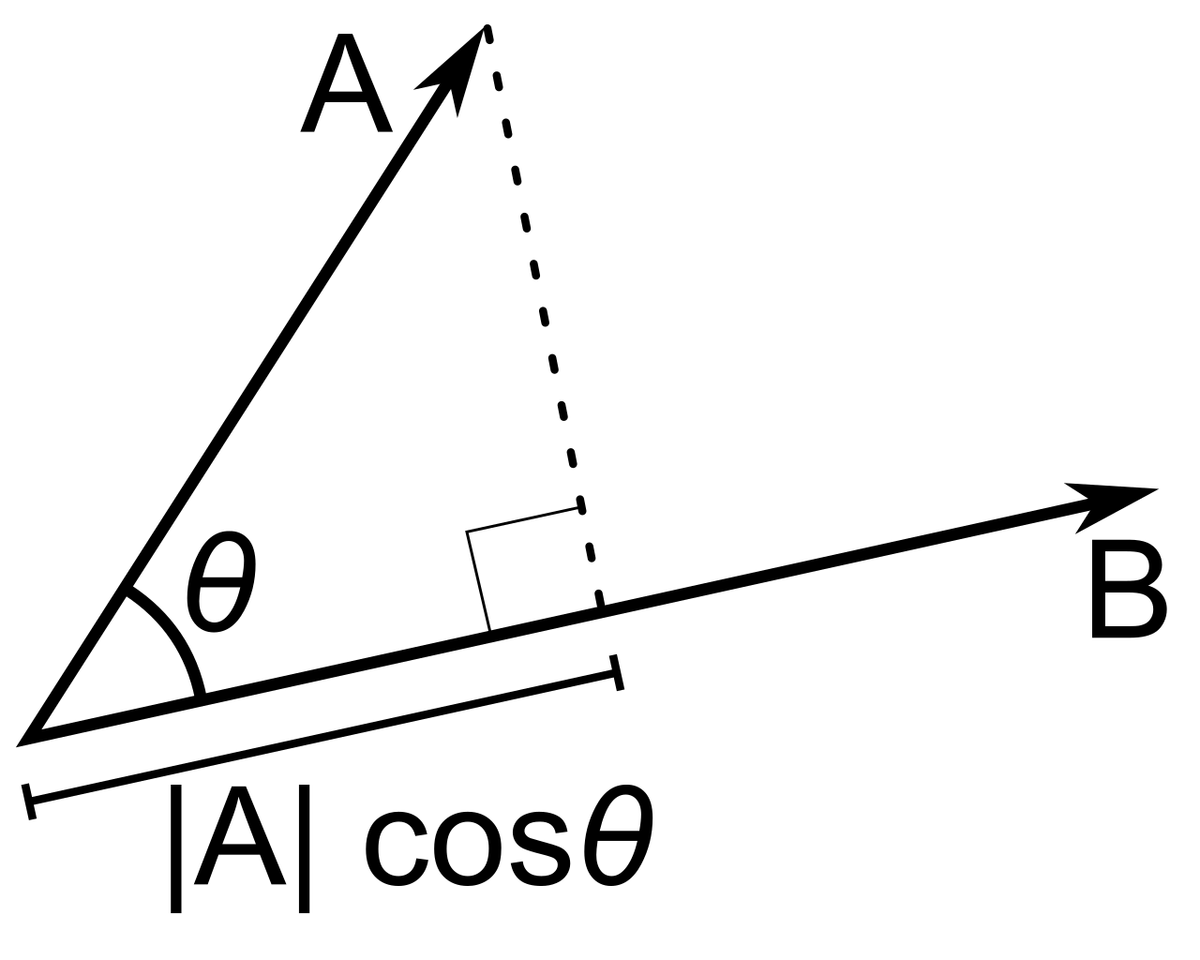
Diagram of vectors A and B separated by the angle theta, showing the scalar projection |A| cos theta of A onto B. No machine-readable author provided. Mazin07 assumed (based on copyright claims)., via Wikimedia Commons, Public domain.
## Definition
### Algebraic definition
For two vectors $\mathbf{x} = (x_1, \ldots, x_n)$ and $\mathbf{y} = (y_1, \ldots, y_n)$ in $\mathbb{R}^n$, the dot product is
$$
\mathbf{x} \cdot \mathbf{y} = x_1 y_1 + x_2 y_2 + \cdots + x_n y_n = \sum_{i=1}^{n} x_i y_i .
$$
The result is a number, not a vector [1]. When vectors are treated as column matrices, the same quantity is written as the matrix product $\mathbf{x}^\top \mathbf{y}$, as in the textbook *Deep Learning* by Goodfellow, Bengio and Courville [2]. Other common notations are $\langle \mathbf{x}, \mathbf{y} \rangle$, used for inner products in general [1], and $\mathbf{x} \cdot \mathbf{y}$, which gives the operation its name [4].
A short example: for $\mathbf{a} = (1, 2, 3)$ and $\mathbf{b} = (4, -5, 6)$,
$$
\mathbf{a} \cdot \mathbf{b} = (1)(4) + (2)(-5) + (3)(6) = 4 - 10 + 18 = 12 .
$$
Taking the dot product of a vector with itself gives the square of its Euclidean length: $\mathbf{x} \cdot \mathbf{x} = \lVert \mathbf{x} \rVert^2$ [1].
### Geometric definition
The dot product can also be written in terms of lengths and angles:
$$
\mathbf{x} \cdot \mathbf{y} = \lVert \mathbf{x} \rVert \, \lVert \mathbf{y} \rVert \cos \theta ,
$$
where $\lVert \cdot \rVert$ is the Euclidean ($L^2$) norm and $\theta$ is the angle between the two vectors [2]. Edwin Bidwell Wilson's 1901 textbook, based on J. Willard Gibbs's lectures, took this form as the definition and then derived the coordinate formula $A_1B_1 + A_2B_2 + A_3B_3$ for three-dimensional vectors written in terms of the unit vectors $\mathbf{i}$, $\mathbf{j}$ and $\mathbf{k}$ [4].
The sign of the dot product follows the angle. It is positive when the angle is less than 90 degrees, zero when the vectors are perpendicular, and negative when the angle is greater than 90 degrees. Two vectors whose dot product is zero are called **orthogonal**; if both have nonzero length, they meet at a right angle, and orthogonal vectors that also have unit length are called **orthonormal** [2]. Dividing the dot product by the two lengths isolates $\cos\theta$, which is the definition of [cosine similarity](https://aiwiki.ai/wiki/cosine_similarity).
A standard physical reading comes from mechanics: the work done by a constant force $\mathbf{A}$ acting through a displacement $\mathbf{B}$ is $\mathbf{A} \cdot \mathbf{B}$ [4].
"Dot products and duality | Chapter 9, Essence of linear algebra", video from 3Blue1Brown, published August 24, 2016. Watch on YouTube.
## Properties
The dot product on $\mathbb{R}^n$ satisfies the following rules [1][2]:
| Property | Statement |
|---|---|
| Commutativity (symmetry) | $\mathbf{x} \cdot \mathbf{y} = \mathbf{y} \cdot \mathbf{x}$ |
| Linearity in each argument | $(a\mathbf{x} + b\mathbf{z}) \cdot \mathbf{y} = a(\mathbf{x} \cdot \mathbf{y}) + b(\mathbf{z} \cdot \mathbf{y})$ |
| Positivity | $\mathbf{x} \cdot \mathbf{x} \ge 0$ |
| Definiteness | $\mathbf{x} \cdot \mathbf{x} = 0$ only when $\mathbf{x} = \mathbf{0}$ |
| Cauchy-Schwarz inequality | $\lvert \mathbf{x} \cdot \mathbf{y} \rvert \le \lVert \mathbf{x} \rVert \, \lVert \mathbf{y} \rVert$ |
Wilson's text proves the distributive law $(\mathbf{A} + \mathbf{B}) \cdot \mathbf{C} = \mathbf{A} \cdot \mathbf{C} + \mathbf{B} \cdot \mathbf{C}$ geometrically, by noting that the projection of a sum equals the sum of the projections [4]. The Cauchy-Schwarz inequality becomes an equality exactly when one vector is a scalar multiple of the other. Axler's textbook credits Augustin-Louis Cauchy with proving the version for sums of products in 1821, and notes that Viktor Bunyakovsky proved integral versions in 1859 before later work by Hermann Schwarz attached his name to the result [1]. The inequality guarantees that the cosine in the geometric definition always lies between -1 and 1.
### Projection
The dot product gives the component of one vector along another. For a nonzero vector $\mathbf{v}$, any vector $\mathbf{u}$ can be split as
$$
\mathbf{u} = c\,\mathbf{v} + \mathbf{w}, \qquad c = \frac{\mathbf{u} \cdot \mathbf{v}}{\lVert \mathbf{v} \rVert^2},
$$
where $\mathbf{w}$ is orthogonal to $\mathbf{v}$ [1]. When $\mathbf{v}$ is a unit vector, $c$ is simply $\mathbf{u} \cdot \mathbf{v}$, the signed length of the shadow that $\mathbf{u}$ casts on the line through $\mathbf{v}$. Wilson's 1901 text describes $\mathbf{A} \cdot \mathbf{c}$, for a unit vector $\mathbf{c}$, as the projection of $\mathbf{A}$ upon $\mathbf{c}$ [4].
### Relation to Euclidean distance
Expanding the squared distance between two vectors with the linearity and symmetry rules gives
$$
\lVert \mathbf{x} - \mathbf{y} \rVert^2 = \lVert \mathbf{x} \rVert^2 + \lVert \mathbf{y} \rVert^2 - 2\,\mathbf{x} \cdot \mathbf{y} .
$$
For unit-length vectors this reduces to $\lVert \mathbf{x} - \mathbf{y} \rVert^2 = 2 - 2\,\mathbf{x} \cdot \mathbf{y}$, so ranking by smallest [Euclidean distance](https://aiwiki.ai/wiki/euclidean_distance), by largest dot product, and by largest cosine similarity all give the same order [9]. Without normalization the three can disagree, which matters for the retrieval systems described below.
## Inner products and complex vectors
An inner product is the abstraction of the dot product to general vector spaces. For real vector spaces, an inner product is any function with the positivity, definiteness, linearity and symmetry properties listed above [1]. For complex vectors the plain sum of products does not work, because $\sum_i z_i z_i$ is not in general a nonnegative real number. The Euclidean inner product on $\mathbb{C}^n$ therefore takes the complex conjugate of one argument, and symmetry is replaced by conjugate symmetry: swapping the arguments conjugates the result [1].
Numerical libraries expose both conventions. The reference BLAS routine ZDOTC computes the conjugated product $\mathbf{x}^H \mathbf{y}$, while ZDOTU computes the unconjugated $\mathbf{x}^\top \mathbf{y}$ [10][11]. In [NumPy](https://aiwiki.ai/wiki/numpy), `numpy.dot` on two one-dimensional arrays returns their inner product without complex conjugation [12], whereas `numpy.vdot` replaces its first argument by its complex conjugate and flattens multidimensional inputs to one dimension before multiplying [13].
## Relation to matrix multiplication
[Matrix multiplication](https://aiwiki.ai/wiki/matrix_multiplication) is built from dot products. In the product $C = AB$, each entry $C_{i,j}$ is the dot product of row $i$ of $A$ with column $j$ of $B$ [2]. Multiplying an $m \times k$ matrix by a $k \times n$ matrix therefore computes $mn$ dot products of length $k$. Unlike matrix multiplication in general, the dot product of two vectors is commutative [2].
Programming interfaces reflect the connection. Python's PEP 465, written by Nathaniel J. Smith and adopted in Python 3.5, added the `@` operator for matrix multiplication; the proposal notes that NumPy users previously wrote `numpy.dot(a, b)` or `a.dot(b)` for this purpose, and it defines `@` applied to two one-dimensional arrays as the standard inner product on vectors [14]. The current NumPy documentation recommends `matmul` or `a @ b` over `numpy.dot` for two-dimensional arrays [12].
## History
In Michael J. Crowe's account of the history of vector analysis, forms of the dot product appear in the 1840s in the work of both Hermann Grassmann and William Rowan Hamilton (in Hamilton's case as the negative of the scalar part of a quaternion product), and the operation reached its modern form in the vector analysis of Gibbs and Heaviside [3].
| Year | Event |
|---|---|
| 1840 | Hermann Grassmann's essay on tidal theory, *Theorie der Ebbe und Flut*, includes a "linear product" of two directed line segments that is identical to the modern dot product [3] |
| 1843 | William Rowan Hamilton discovers quaternions on 16 October [3] |
| 1844 | Grassmann's *Die lineale Ausdehnungslehre* introduces inner and outer products, close to the modern dot and cross products [3] |
| 1846 | Hamilton introduces the terms "scalar" and "vector" for the real and imaginary parts of a quaternion [3] |
| 1881 | J. Willard Gibbs prints the first half of *Elements of Vector Analysis* [3] |
| 1884 | Gibbs prints the second half [3] |
| 1885 | Oliver Heaviside gives his first unified presentation of a vector system essentially identical to Gibbs's [3] |
| 1901 | Edwin Bidwell Wilson publishes *Vector Analysis*, founded on Gibbs's lectures [4] |
In Hamilton's quaternion algebra, multiplying two quaternions whose scalar parts are zero, $Q = xi + yj + zk$ and $Q' = x'i + y'j + z'k$, gives a quaternion whose scalar part is $-(xx' + yy' + zz')$, the negative of the modern dot product, and whose vector part equals the modern cross product. Crowe identifies this as the path along which modern vector analysis originated [3]. Gibbs and Heaviside, working independently, developed the system of vector analysis that is now almost universally taught [3], in which the dot product and the cross product are defined as two separate products of vectors [4].
Gibbs's *Elements of Vector Analysis* was printed as a pamphlet in 1881 to 1884 and, in his words, never published, though it circulated among people interested in the subject [4]. Wilson's 1901 book, which Crowe describes as the first book-length, formally published presentation of modern vector analysis in English [3], defines the "direct product" of two vectors as the product of their magnitudes and the cosine of the angle between them. It writes the product with a dot between the vectors, says it is read "A dot B" and may therefore be called the dot product, and adds that it is also called the scalar product because its value is a scalar [4]. Wilson's preface says the book also drew on the vector analysis chapters in Heaviside's *Electromagnetic Theory* (1893) [4].
## Role in machine learning
### Neurons and fully connected layers
A typical hidden unit in a feedforward network takes an input vector $\mathbf{x}$, computes an affine transformation, and applies a nonlinear [activation function](https://aiwiki.ai/wiki/activation_function). For hidden unit $i$ with weight column $W_{:,i}$ and bias $c_i$, the output is $h_i = g(\mathbf{x}^\top W_{:,i} + c_i)$ [5]. The term inside $g$ is a dot product plus a [bias](https://aiwiki.ai/wiki/bias), in other words a [weighted sum](https://aiwiki.ai/wiki/weighted_sum) of the inputs. A whole layer stacks these dot products into one matrix-vector product, and a minibatch of inputs turns it into a matrix-matrix product.
The same pattern appears in [linear regression](https://aiwiki.ai/wiki/linear_regression), which maps an input vector to an output scalar with a vector of weights and a scalar bias, $\mathbf{w}^\top \mathbf{x} + b$ [5]. [Backpropagation](https://aiwiki.ai/wiki/backpropagation) also relies on dot products: the gradient with respect to a node is computed as a dot product between gradients already computed for its children and the partial derivatives connecting them [5].
### Convolution
A [convolutional neural network](https://aiwiki.ai/wiki/convolutional_neural_network) slides a small kernel over its input. Many neural network libraries implement this as cross-correlation, $S(i, j) = \sum_m \sum_n I(i + m, j + n) K(m, n)$, and call it convolution [15]. Each output value is therefore the dot product between the kernel weights and the input patch under the kernel at that position, so a [convolutional filter](https://aiwiki.ai/wiki/convolutional_filter) is a set of weights that is dotted with every patch of its input.
### Attention
Attention layers compute a score between a query and each position it can attend to, then turn the scores into weights with a [softmax](https://aiwiki.ai/wiki/softmax) [16][6]. Luong, Pham and Manning's 2015 study of attention for [neural machine translation](https://aiwiki.ai/wiki/neural_machine_translation) compared three content-based score functions between a decoder state $\mathbf{h}_t$ and an encoder state $\bar{\mathbf{h}}_s$: **dot** ($\mathbf{h}_t^\top \bar{\mathbf{h}}_s$), **general** ($\mathbf{h}_t^\top W_a \bar{\mathbf{h}}_s$) and **concat** ($\mathbf{v}_a^\top \tanh(W_a[\mathbf{h}_t; \bar{\mathbf{h}}_s])$). They noted that Bahdanau and colleagues' earlier model had used only the concat form, and reported that dot worked well for global attention while general was better for local attention [16].
The 2017 paper "[Attention Is All You Need](https://aiwiki.ai/wiki/attention_is_all_you_need)" built the Transformer around **scaled dot-product attention** [6]:
$$
\mathrm{Attention}(Q, K, V) = \mathrm{softmax}\!\left(\frac{QK^\top}{\sqrt{d_k}}\right) V ,
$$
where the rows of $Q$, $K$ and $V$ are query, key and value vectors and $d_k$ is the key dimension. Each entry of $QK^\top$ is the dot product of one query with one key. The authors named additive and dot-product (multiplicative) attention as the two most common attention functions and wrote that dot-product attention is much faster and more space-efficient in practice because it can use highly optimized matrix multiplication code [6]. They also reported that additive attention outperforms dot-product attention without scaling for larger $d_k$, and suspected the cause was dot products growing large in magnitude and pushing the softmax into regions with extremely small gradients. A footnote gives the reasoning: if the components of a query and a key are independent random variables with mean 0 and variance 1, their dot product has mean 0 and variance $d_k$, so dividing by $\sqrt{d_k}$ restores unit variance [6].
The base Transformer used $h = 8$ heads with $d_k = 64$ per head [6]. Because every query is compared with every key, a self-attention layer costs $O(n^2 \cdot d)$ for a sequence of length $n$ and representation size $d$, which the paper lists in its complexity comparison with recurrent and convolutional layers [6]. Decoder self-attention blocks future positions by setting their scores to $-\infty$ before the softmax [6]. See [self-attention](https://aiwiki.ai/wiki/self_attention) and [Flash Attention](https://aiwiki.ai/wiki/flash_attention) for how these dot products are batched and computed efficiently.
### Similarity search and dense retrieval
In embedding-based search, documents and queries are mapped to vectors and the system returns the documents whose vectors score highest against the query. Dense Passage Retrieval (DPR), a 2020 open-domain question answering system, defines the similarity between a question $q$ and a passage $p$ as the dot product $E_Q(q)^\top E_P(p)$ of two [BERT](https://aiwiki.ai/wiki/bert) encoders' outputs [7]. The authors noted that cosine similarity is equivalent to the inner product for unit vectors. In their ablations, Euclidean distance performed comparably to the dot product and both were better than cosine similarity, so they kept the simpler inner product [7]. DPR outperformed BM25 by a large margin, with 65.2% versus 42.9% top-5 retrieval accuracy [7].
Finding the stored vectors with the largest dot product to a query is called **maximum inner product search** (MIPS). Shrivastava and Li argued in 2014 that the existing locality-sensitive hashing framework was insufficient for MIPS, and proposed asymmetric hashing, which applies different transformations to queries and to stored items so that the problem becomes approximate near-neighbor search; they evaluated it on item recommendation with Netflix and MovieLens data [17]. Google's ScaNN library implements MIPS with search space pruning and quantization [18]. Its quantization method, published at ICML 2020, starts from the observation that the database points with the largest inner products to a query matter most, and uses an anisotropic loss that penalizes the part of a data point's quantization error parallel to the point more heavily than the orthogonal part [19][18].
The [FAISS](https://aiwiki.ai/wiki/faiss) similarity search library documents the practical consequences. Its inner-product metric is typically used for MIPS in recommendation systems; the norm of the query does not change the ranking of results, but the norms of the database vectors do. To search by cosine similarity, users normalize both the database and query vectors and then search by inner product [9]. The [Sentence Transformers](https://aiwiki.ai/wiki/sentence_transformers) library makes cosine similarity its default, notes that the dot product of normalized embeddings is equivalent and faster, and advises choosing the dot product when a model ends with a normalization module [20].
### Recommendation systems
[Matrix factorization](https://aiwiki.ai/wiki/matrix_factorization) methods for [collaborative filtering](https://aiwiki.ai/wiki/collaborative_filtering) in [recommendation systems](https://aiwiki.ai/wiki/recommendation_system) represent each user $u$ by a vector $\mathbf{p}_u$ and each item $i$ by a vector $\mathbf{q}_i$ in a shared latent factor space. In Koren, Bell and Volinsky's description, the dot product $\mathbf{q}_i^\top \mathbf{p}_u$ captures the interaction between the user and the item, the user's overall interest in the item's characteristics, and approximates the user's rating of the item [21]. The same article opens by stating that the [Netflix Prize](https://aiwiki.ai/wiki/netflix_prize) competition had shown matrix factorization models to be superior to classic nearest-neighbor techniques for product recommendations [21].
### Contrastive learning
[Contrastive learning](https://aiwiki.ai/wiki/contrastive_learning) methods train encoders so that matching pairs have high similarity scores. [CLIP](https://aiwiki.ai/wiki/clip) computes its training logits by L2-normalizing image and text embeddings and taking the dot product of every image embedding with every text embedding in a batch, which the paper's pseudocode labels "scaled pairwise cosine similarities". The scores are multiplied by a learned temperature, initialized to the equivalent of 0.07 and clipped so that logits are never scaled by more than 100 [22].
### Kernel methods
Cortes and Vapnik's 1995 paper "Support-Vector Networks", which extended the earlier separable-data version of what are now called [support vector machines](https://aiwiki.ai/wiki/support_vector_machine_svm) to training data that cannot be separated without errors, observed that the classification function for an input in a transformed feature space depends only on dot products, and replaced those dot products with a function $K(\mathbf{u}, \mathbf{v})$ satisfying Mercer's condition, a step the paper calls the "convolution of the dot-product" [23]. Citing Boser, Guyon and Vapnik (1992), the paper notes that different choices of $K$ yield different learning machines, and it gives polynomial and radial basis function machines as examples [23]. See [kernel trick](https://aiwiki.ai/wiki/kernel_trick) for the general technique.
### Dot product versus cosine similarity
Whether to compare embeddings by raw dot product or by cosine similarity is a recurring design choice. The dot product depends on the lengths of the vectors as well as on the angle between them, while cosine similarity depends only on the angle. Steck, Ekanadham and Kallus reported in 2024 that cosine similarity sometimes works better and sometimes worse than the unnormalized dot product on learned embeddings. Analyzing regularized linear models, they showed that cosine similarities can be non-unique or implicitly controlled by the choice of regularization, and so can produce arbitrary results; they cautioned against using cosine similarity blindly [24]. DPR's ablation, in which the dot product beat cosine similarity for passage retrieval, is one empirical data point on the same question [7].
## Computation
### Software
The Basic Linear Algebra Subprograms (BLAS) trace back to a 1979 paper by Lawson, Hanson, Kincaid and Krogh in *ACM Transactions on Mathematical Software* [25]. The reference BLAS group vector-vector operations such as the dot product into Level 1, matrix-vector operations into Level 2, and matrix-matrix operations into Level 3 [26]. The reference implementation's DDOT routine forms the dot product of two double-precision vectors and uses unrolled loops when the vectors are stored contiguously [27]. Array libraries expose the operation directly: [PyTorch](https://aiwiki.ai/wiki/pytorch)'s `torch.dot` computes the dot product of two one-dimensional tensors with the same number of elements and, unlike NumPy's `dot`, intentionally supports only that case [28].
### Hardware and numerical precision
A dot product of length $n$ takes $n$ multiplications and $n - 1$ additions, which can be carried out as a chain of multiply-accumulate (MAC) operations. Google's [Tensor Processing Unit](https://aiwiki.ai/wiki/tpu) (TPU), as described in a 2017 paper, centers on a matrix multiply unit of 65,536 8-bit MACs with a peak throughput of 92 tera-operations per second [29]. NVIDIA's Volta GPUs introduced [Tensor Cores](https://aiwiki.ai/wiki/tensor_core) that multiply FP16 input matrices and accumulate the products into FP16 or FP32 outputs [8].
Numerical precision also matters. In their 2018 paper on [mixed-precision training](https://aiwiki.ai/wiki/mixed_precision_training), Micikevicius and colleagues found that some networks only matched full-precision accuracy if FP16 vector dot products accumulated their partial products into an FP32 value, which is converted back to FP16 before being written to memory [8]. See [floating point](https://aiwiki.ai/wiki/floating_point) and [FP16](https://aiwiki.ai/wiki/fp16) for the number formats involved.
## See also
- [Cosine similarity](https://aiwiki.ai/wiki/cosine_similarity)
- [Matrix multiplication](https://aiwiki.ai/wiki/matrix_multiplication)
- [Weighted sum](https://aiwiki.ai/wiki/weighted_sum)
- [Scalar](https://aiwiki.ai/wiki/scalar)
- [Attention](https://aiwiki.ai/wiki/attention)
- [Embedding vector](https://aiwiki.ai/wiki/embedding_vector)
- [Approximate nearest-neighbor search](https://aiwiki.ai/wiki/approximate_nearest_neighbor_search)
- [Linear algebra](https://aiwiki.ai/wiki/linear_algebra)
## References
1. Axler, Sheldon. "Linear Algebra Done Right" (fourth edition), Chapter 6: Inner Product Spaces. Springer (open access), 2024. https://linear.axler.net/LADR4e.pdf
2. Goodfellow, Ian; Bengio, Yoshua; Courville, Aaron. "Linear Algebra" (Chapter 2). Deep Learning, MIT Press, 2016. https://www.deeplearningbook.org/contents/linear_algebra.html
3. Crowe, Michael J. "A History of Vector Analysis". Lecture text, University of Louisville, Autumn 2002. https://www.math.ucdavis.edu/~temple/MAT21D/SUPPLEMENTARY-ARTICLES/Crowe_History-of-Vectors.pdf
4. Wilson, Edwin Bidwell. "Vector Analysis: A Text-Book for the Use of Students of Mathematics and Physics, Founded upon the Lectures of J. Willard Gibbs". Charles Scribner's Sons (Yale Bicentennial Publications), New York, 1901. https://archive.org/details/vectoranalysiste00gibbiala
5. Goodfellow, Ian; Bengio, Yoshua; Courville, Aaron. "Deep Feedforward Networks" (Chapter 6). Deep Learning, MIT Press, 2016. https://www.deeplearningbook.org/contents/mlp.html
6. Vaswani, Ashish; Shazeer, Noam; Parmar, Niki; Uszkoreit, Jakob; Jones, Llion; Gomez, Aidan N.; Kaiser, Lukasz; Polosukhin, Illia. "Attention Is All You Need". arXiv:1706.03762, 2017. https://arxiv.org/abs/1706.03762
7. Karpukhin, Vladimir; Oğuz, Barlas; Min, Sewon; Lewis, Patrick; Wu, Ledell; Edunov, Sergey; Chen, Danqi; Yih, Wen-tau. "Dense Passage Retrieval for Open-Domain Question Answering". EMNLP 2020; arXiv:2004.04906. https://arxiv.org/abs/2004.04906
8. Micikevicius, Paulius; Narang, Sharan; Alben, Jonah; Diamos, Gregory; Elsen, Erich; Garcia, David; Ginsburg, Boris; Houston, Michael; Kuchaiev, Oleksii; Venkatesh, Ganesh; Wu, Hao. "Mixed Precision Training". ICLR 2018; arXiv:1710.03740. https://arxiv.org/abs/1710.03740
9. Meta AI Research (facebookresearch/faiss). "MetricType and distances". Faiss wiki, GitHub. https://github.com/facebookresearch/faiss/wiki/MetricType-and-distances
10. Netlib. "ZDOTC" (reference BLAS source, zdotc.f). Netlib Repository. https://netlib.org/blas/zdotc.f
11. Netlib. "ZDOTU" (reference BLAS source, zdotu.f). Netlib Repository. https://netlib.org/blas/zdotu.f
12. NumPy Developers. "numpy.dot". NumPy v2.5 Manual. https://numpy.org/doc/stable/reference/generated/numpy.dot.html
13. NumPy Developers. "numpy.vdot". NumPy v2.5 Manual. https://numpy.org/doc/stable/reference/generated/numpy.vdot.html
14. Smith, Nathaniel J. "PEP 465: A dedicated infix operator for matrix multiplication". Python Enhancement Proposals, created 2014-02-20. https://peps.python.org/pep-0465/
15. Goodfellow, Ian; Bengio, Yoshua; Courville, Aaron. "Convolutional Networks" (Chapter 9). Deep Learning, MIT Press, 2016. https://www.deeplearningbook.org/contents/convnets.html
16. Luong, Minh-Thang; Pham, Hieu; Manning, Christopher D. "Effective Approaches to Attention-based Neural Machine Translation". EMNLP 2015; arXiv:1508.04025. https://arxiv.org/abs/1508.04025
17. Shrivastava, Anshumali; Li, Ping. "Asymmetric LSH (ALSH) for Sublinear Time Maximum Inner Product Search (MIPS)". Neural Information Processing Systems (NIPS) 2014; arXiv:1405.5869. https://arxiv.org/abs/1405.5869
18. Google Research. "ScaNN" (README). google-research repository, GitHub. https://github.com/google-research/google-research/tree/master/scann
19. Guo, Ruiqi; Sun, Philip; Lindgren, Erik; Geng, Quan; Simcha, David; Chern, Felix; Kumar, Sanjiv. "Accelerating Large-Scale Inference with Anisotropic Vector Quantization". International Conference on Machine Learning (ICML) 2020; arXiv:1908.10396. https://arxiv.org/abs/1908.10396
20. Sentence Transformers. "Semantic Textual Similarity". Sentence Transformers documentation. https://sbert.net/docs/sentence_transformer/usage/semantic_textual_similarity.html
21. Koren, Yehuda; Bell, Robert; Volinsky, Chris. "Matrix Factorization Techniques for Recommender Systems". Computer 42(8): 30-37, IEEE, August 2009. https://doi.org/10.1109/MC.2009.263
22. Radford, Alec; Kim, Jong Wook; Hallacy, Chris; Ramesh, Aditya; Goh, Gabriel; Agarwal, Sandhini; Sastry, Girish; Askell, Amanda; Mishkin, Pamela; Clark, Jack; Krueger, Gretchen; Sutskever, Ilya. "Learning Transferable Visual Models From Natural Language Supervision". arXiv:2103.00020, 2021. https://arxiv.org/abs/2103.00020
23. Cortes, Corinna; Vapnik, Vladimir. "Support-Vector Networks". Machine Learning 20: 273-297, 1995. https://doi.org/10.1007/BF00994018
24. Steck, Harald; Ekanadham, Chaitanya; Kallus, Nathan. "Is Cosine-Similarity of Embeddings Really About Similarity?". ACM Web Conference 2024 (WWW 2024 Companion); arXiv:2403.05440. https://arxiv.org/abs/2403.05440
25. Lawson, C. L.; Hanson, R. J.; Kincaid, D. R.; Krogh, F. T. "Basic Linear Algebra Subprograms for Fortran Usage". ACM Transactions on Mathematical Software 5(3): 308-323, September 1979. https://doi.org/10.1145/355841.355847
26. Netlib. "BLAS (Basic Linear Algebra Subprograms)". Netlib Repository. https://netlib.org/blas/
27. Netlib. "DDOT" (reference BLAS source, ddot.f). Netlib Repository. https://netlib.org/blas/ddot.f
28. PyTorch Contributors. "torch.dot". PyTorch 2.15 documentation. https://docs.pytorch.org/docs/2.15/generated/torch.dot.html
29. Jouppi, Norman P.; Young, Cliff; Patil, Nishant; Patterson, David; et al. "In-Datacenter Performance Analysis of a Tensor Processing Unit". 44th International Symposium on Computer Architecture (ISCA), 2017; arXiv:1704.04760. https://arxiv.org/abs/1704.04760