# Statistical hypothesis testing
> Source: https://aiwiki.ai/wiki/hypothesis_testing
> Updated: 2026-11-18
> Fact-checked: 2026-11-18
> Categories: Machine Learning, Model Evaluation, Statistics
> License: CC BY 4.0 (https://creativecommons.org/licenses/by/4.0/) - attribute to "AI Wiki (aiwiki.ai)"
> Cite as: AI Wiki. "Statistical hypothesis testing." aiwiki.ai, 18 Nov 2026. https://aiwiki.ai/wiki/hypothesis_testing
> From AI Wiki (https://aiwiki.ai), the free encyclopedia of artificial intelligence. Reuse freely with attribution.
**Statistical hypothesis testing** is a family of procedures for deciding, from sample data, whether there is enough evidence to reject a stated conjecture about a process or population, called the null hypothesis, in favor of an alternative.[1] A test computes a statistic from the data and compares it with what that statistic would look like if the null hypothesis were true, either through a critical value or through a p-value.[2] The modern framework was developed mainly in the first half of the twentieth century, building on work by Karl Pearson and "Student" and formalized in different ways by Ronald Fisher and by Jerzy Neyman and Egon Pearson.[3][5][6] In [machine learning](https://aiwiki.ai/wiki/machine_learning), hypothesis tests are used to judge whether one model really outperforms another on a [benchmark](https://aiwiki.ai/wiki/benchmark) or whether the gap could be explained by the particular test examples, random seeds and training runs that happened to be used.[14][15][22] The method has also drawn sustained criticism, including a 2016 statement on p-values by the American Statistical Association and proposals to tighten or abandon fixed significance thresholds.[9][10][11]
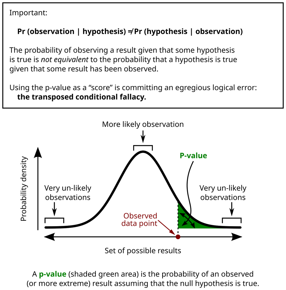
Illustration of a p-value as the probability, under the null hypothesis, of a result at least as extreme as the one observed (the shaded tail area). Via Wikimedia Commons, CC BY-SA 3.0.
## Core concepts
### Null and alternative hypotheses
A test needs a pair of hypotheses: a null hypothesis $H_0$ and an alternative hypothesis $H_a$ (also written $H_1$).[1] The NIST/SEMATECH e-Handbook of Statistical Methods illustrates this with a photomask production line, where the null hypothesis is that the mean linewidth equals 500 micrometers and the alternative is that it does not. Because that alternative guards against deviations in both directions, it is called two-sided. A one-sided alternative guards against a deviation in only one direction, as when a test of light bulbs takes as its null hypothesis that the mean lifetime is at least 500 hours and rejects only if the evidence points to a shorter lifetime.[1]
Failing to reject the null hypothesis is not the same as proving it. The NIST handbook notes that a non-rejection may simply mean that there are not yet enough data to reject.[1]
### Test statistic, critical values and p-values
A test statistic is a number computed from the sample, and its form is specific to the type of test. Critical values are cut-off points that mark a rejection region: values of the statistic that would be unlikely if the null hypothesis were true. If the observed statistic falls in that region, the null hypothesis is rejected.[2]
The p-value is the probability, computed under the null hypothesis, of obtaining a test statistic at least as extreme as the one actually observed.[2] For a test in which large values of a statistic $T$ count as extreme,
$$p = P\left(T \ge t_{\text{obs}} \mid H_0\right),$$
where $t_{\text{obs}}$ is the value computed from the data. A small p-value means that a result like the one observed would be unlikely if the null hypothesis were true, and NIST treats it as an indication that the null hypothesis is false.[2] NIST describes it as good practice to decide in advance how small a p-value must be to reject, which is equivalent to choosing a significance level before the test.[2]
The Stanford Encyclopedia of Philosophy's entry on the philosophy of statistics illustrates the logic with a version of Fisher's tea-tasting experiment. A student claims to be able to tell whether milk or tea was poured into a cup first. Five cups are prepared in random order and the student names the order correctly every time. If the student were guessing, each answer would be right with probability 1/2, so five correct answers would occur with probability $1/2^5$, about 3%, which can be taken as grounds to reject the guessing hypothesis.[3] The same entry cautions that "the p-value is unfortunately ill-understood by statistical practitioners."[3]
### Errors, significance level and power
A test can go wrong in two ways.[3]
| | $H_0$ is true | $H_0$ is false |
|---|---|---|
| Reject $H_0$ | Type I error ([false positive](https://aiwiki.ai/wiki/false_positive)), probability $\alpha$ | Correct decision, probability $1-\beta$ (power) |
| Fail to reject $H_0$ | Correct decision ([true negative](https://aiwiki.ai/wiki/true_negative)), probability $1-\alpha$ | Type II error ([false negative](https://aiwiki.ai/wiki/false_negative)), probability $\beta$ |
A Type I error is the rejection of a null hypothesis that is in fact true. Its probability, $\alpha$, is also called the significance level of the test. A Type II error is the acceptance of the null hypothesis when the alternative is true; its probability is written $\beta$, and $1-\beta$ is called the power of the test.[3] NIST notes that a value of $\alpha = 0.05$ means the null hypothesis is rejected 5% of the time when it is true, that the choice of $\alpha$ is "somewhat arbitrary", and that 0.1, 0.05 and 0.01 are common in practice.[2]
The two error rates pull against each other. The Type II error rate is not chosen directly by the analyst: it depends on how far reality is from the null hypothesis, with large discrepancies easier to detect than small ones, and it rises as $\alpha$ is made smaller.[1] Power analysis turns this around and asks how large a sample is needed to detect an effect of a given size with a given probability. In natural language processing research, Card and colleagues describe an experiment as underpowered when it has too few subjects or items, a threshold often taken to be less than 80% power.[18]
"Hypothesis Testing and The Null Hypothesis, Clearly Explained!!!", video from StatQuest with Josh Starmer, published July 6, 2020. Watch on YouTube.
## History
| Year | Contribution | Source |
|---|---|---|
| 1710 | John Arbuthnot compares male and female christenings in London | [7] |
| 1900 | Karl Pearson establishes the distribution of the $\chi^2$ statistic | [5] |
| 1908 | "Student" gives the distributions needed for small-sample tests of means | [6] |
| 1925 | Ronald Fisher's *Statistical Methods for Research Workers* treats P = .05 as a convenient limit | [4][5] |
| 1933 | Neyman and Pearson publish their paper on most efficient tests | [8] |
| 2016 | American Statistical Association issues a statement on p-values | [9] |
### Early significance arguments
John Arbuthnot's 1710 paper in the *Philosophical Transactions of the Royal Society* is described in the documentation of the R package HistData as the first known significance test. Arbuthnot used London christening records from 1629 to 1710, in which male christenings outnumbered female ones in every year, and showed that such a run would be vanishingly unlikely (about $4.14 \times 10^{-25}$) if male and female births were equally likely. He took this as evidence of divine providence.[7] Later analysts have pointed out that his figures count public baptisms rather than births and contain at least one year copied from another.[7]
By Fisher's account, the distribution of the $\chi^2$ statistic was established by Karl Pearson in 1900, which made it possible to calculate how often any given value of $\chi^2$ would be exceeded.[5] In 1908 the statistician writing as "Student" pointed out that with small samples, of the kind usual in field and laboratory experiments, the population variance can only be roughly estimated from the sample, and gave the distributions needed to allow for this. Fisher's book gave these distributions, in a form similar to its table of $\chi^2$, in a table of $t$ at the end of the chapter.[6]
### Fisher and the 5% convention
Ronald Fisher's *Statistical Methods for Research Workers* (1925) called procedures for deciding whether a second sample differs from a first "tests of significance".[4] Discussing the normal distribution, Fisher observed that the deviation for which P = .05 is 1.96, or nearly 2 standard deviations, and wrote that "it is convenient to take this point as a limit in judging whether a deviation is to be considered significant or not."[4] In the chapter on $\chi^2$ he added that "we shall not often be astray if we draw a conventional line at .05".[5] In the same chapter he wrote that in practice the first question is whether an observed $\chi^2$ is open to suspicion, not its exact value of P.[5]
### Neyman and Pearson
Jerzy Neyman and Egon Pearson developed a different formulation in papers from 1928 and 1933, including "On the problem of the most efficient tests of statistical hypotheses", published in the *Philosophical Transactions of the Royal Society of London, Series A* in 1933.[3][8] Their approach weighs a null hypothesis against an explicit alternative and is organized around the two error rates. An optimal test minimizes both errors, and the fundamental lemma of Neyman and Pearson shows that a test has optimal significance and power exactly when it is a likelihood-ratio test, which rejects according to a threshold on the ratio of the probability of the data under the alternative to its probability under the null.[3]
### Two interpretations
The Stanford Encyclopedia of Philosophy contrasts the two traditions. In its presentation, the Fisher-style test is stated in terms of the null hypothesis alone, while the Neyman-Pearson test adds an explicit alternative hypothesis and compares the two. Neyman in particular became known for a strictly behaviorist reading, in which error probabilities give no advice about what to believe but state how often one would err in the long run by following the procedure. Fisher, Pearson and other classical statisticians argued instead for more epistemic interpretations, in which a test result bears on the evidence for a hypothesis.[3]
## Common tests
Many tests exist, and the right one depends on how the data were collected and what assumptions they can bear. Parametric tests assume a known distribution for the test statistic under the null hypothesis; non-parametric tests drop that assumption, usually at some cost in power when the parametric assumptions do hold.[15]
| Test | Typical use | Null hypothesis | Source |
|---|---|---|---|
| Paired t-test | Two systems scored on the same items or data sets | The paired samples have the same mean | [15][28] |
| Wilcoxon signed-rank test | Non-parametric alternative to the paired t-test | Differences are symmetric about zero | [14][29] |
| Sign test | Counting wins and losses between two systems | Each system is equally likely to win on an item | [14][15] |
| McNemar's test | Two classifiers on the same examples, scored right or wrong | Both are correct on the same proportion of items | [15] |
| Chi-squared test | Observed versus expected counts | Counts follow the hypothesized proportions | [5] |
| Permutation (randomization) test | Any statistic, few distributional assumptions | Samples come from the same distribution, or pairings are random | [15][30] |
| Paired bootstrap test | Corpus-level metrics such as [BLEU](https://aiwiki.ai/wiki/bleu_bilingual_evaluation_understudy) | No difference between the paired systems | [15][16] |
| Friedman test with post-hoc tests | Several classifiers across several data sets | All algorithms are equivalent (equal average ranks) | [14] |
## Multiple comparisons
Running many tests inflates the chance that some will come out significant by accident. Demšar, writing about classifier comparisons, notes that when many tests are made a certain proportion of null hypotheses will be rejected by chance alone, and that the usual goal is to control the family-wise error rate, the probability of making at least one Type I error across all of the comparisons.[14] The Bonferroni-Dunn procedure does this by dividing $\alpha$ by the number of comparisons; Demšar describes such corrections as generally conservative, with little power.[14]
A less strict target is the false discovery rate, the expected proportion of rejected null hypotheses that are actually true. Yoav Benjamini and Yosef Hochberg introduced a procedure for controlling it in a 1995 paper in the *Journal of the Royal Statistical Society, Series B*, and the SciPy documentation notes that false discovery rate procedures tend to have higher power than family-wise procedures such as the Bonferroni correction.[27] The Python libraries SciPy and statsmodels both implement these adjustments; statsmodels' `multipletests` function offers Bonferroni, Šidák, Holm, Simes-Hochberg, Hommel, Benjamini-Hochberg and Benjamini-Yekutieli adjustments, along with two-stage and adaptive false discovery rate methods.[27][31]
## Use in machine learning evaluation
### Comparing classifiers
According to Benavoli and colleagues, the machine learning community adopted null hypothesis significance testing to validate claims that one method beats another, starting with work by Dietterich (1998) and Salzberg (1997) and followed by Demšar (2006).[26] In his 2006 review in the *Journal of Machine Learning Research*, Janez Demšar summarized Thomas Dietterich's 1998 analysis of tests for comparing two algorithms on a single data set: Dietterich recommended a 5x2 [cross-validation](https://aiwiki.ai/wiki/cross-validation) t-test because the traditional paired t-test over k-fold cross-validation folds underestimates variance and so has an elevated Type I error rate, found McNemar's test about as powerful where running the algorithms many times is impractical, and warned against t-tests after repeated random resampling or cross-validation.[14]
Demšar then examined the harder case of several algorithms compared over many data sets. Reviewing papers from the International Conference on Machine Learning between 1999 and 2003, he found that many ended with pairwise tests between every pair of classifiers and that the Bonferroni correction was used in only a few papers a year.[14] He argued that a paired t-test across data sets is questionable because differences in accuracy on different data sets are not necessarily commensurate, and recommended the Wilcoxon signed-ranks test for comparing two classifiers and the Friedman test with post-hoc tests for comparing more, with results drawn as critical difference (CD) diagrams.[14]
### Natural language processing
In [machine translation](https://aiwiki.ai/wiki/machine_translation), Philipp Koehn's 2004 paper at the Conference on Empirical Methods in Natural Language Processing (EMNLP) introduced paired bootstrap resampling for corpus-level metrics such as BLEU, for which no simple analytical significance test is available. The method repeatedly draws test sets with replacement from the original test set, scores both systems on each, and concludes that one system is better at the 95% level if it wins on 95% of the resampled sets. Koehn reported that the method could give assurances that differences were real even with test sets of only 300 sentences.[16] Berg-Kirkpatrick, Burkett and Klein's 2012 study across several NLP tasks found that systems with more similar outputs reach significance with smaller metric gains, and that test set size has the largest effect on a test's ability to detect differences, though with diminishing returns.[17]
Rotem Dror and colleagues' 2018 guide at the Annual Meeting of the Association for Computational Linguistics (ACL) proposed a decision procedure for choosing among parametric and non-parametric tests in NLP. Surveying the 180 experimental long papers at ACL 2017, they found that only 63 reported a significance test, that 21 of those did not name the test used, and that 6 of the 42 that did named a test they judged inappropriate. Of 33 experimental papers in the journal *Transactions of the Association for Computational Linguistics*, 15 did not include significance testing.[15]
Card and colleagues, writing at EMNLP 2020, argued that statistical power had been largely ignored in NLP. They defined statistical power as the probability that an experiment will reject the null hypothesis given a real effect and concluded that underpowered experiments are common in NLP. They reported that for several tasks in the [GLUE benchmark](https://aiwiki.ai/wiki/glue_benchmark), small test sets mean that most attempted comparisons with state-of-the-art models are not adequately powered, and that typical machine translation test sets of 2,000 sentences have about 75% power to detect a difference of 1 BLEU point.[18]
### Variance from training runs
Test-set sampling is not the only source of noise. Henderson and colleagues argued in a paper accepted to AAAI 2018 that non-determinism in benchmark environments and variance intrinsic to deep [reinforcement learning](https://aiwiki.ai/wiki/reinforcement_learning) methods make reported results hard to interpret, and that without significance metrics and tighter reporting standards it is difficult to tell whether improvements are meaningful.[19] Bouthillier and colleagues modeled the whole benchmarking pipeline and found that data sampling, parameter initialization and [hyperparameter](https://aiwiki.ai/wiki/hyperparameter) choice all markedly affect results. They recommended randomizing as many of these sources of variation as possible and deciding whether algorithm A beats algorithm B by estimating the probability that A outperforms B across runs rather than by comparing average scores alone. In their simulations, comparing a single run of each algorithm produced roughly 10% false positives and 75% false negatives.[20]
Agarwal and colleagues, in a 2021 paper that received an Outstanding Paper Award at NeurIPS, showed on the Atari 100k benchmark that conclusions drawn from point estimates of aggregate performance can differ substantially from those of a more careful statistical analysis when only a few training runs per task are available. They advocated reporting interval estimates, performance profiles and the interquartile mean, and released an open-source library, rliable, for these analyses.[21]
### Large language model evaluations
With [large language models](https://aiwiki.ai/wiki/large_language_model), hypothesis testing has been applied to benchmark scores themselves. In a November 2024 paper, Evan Miller of [Anthropic](https://aiwiki.ai/wiki/anthropic) treated evaluation questions as a sample drawn from an unseen super-population and made five recommendations: compute standard errors of the mean using the central limit theorem; use clustered standard errors when questions come in related groups; reduce variance by resampling answers and by using next-token probabilities; compare two models with inference on question-level paired differences rather than on overall scores; and use power analysis to decide whether an evaluation can test the hypothesis of interest.[22] In the paper's own table of evaluations run with Anthropic models, clustered standard errors ranged from 1.10 times the naive ones on RACE-H to 3.05 times on DROP.[22] Because two models' scores on the same questions tend to be positively correlated, the variance of a paired comparison is smaller than that of an unpaired one:
$$\operatorname{Var}\left(\hat{\mu}_{A-B}^{\text{paired}}\right) = \frac{\operatorname{Var}(s_A) + \operatorname{Var}(s_B) - 2\operatorname{Cov}(s_A, s_B)}{n},$$
where $s_A$ and $s_B$ are the two models' scores on a question and $n$ is the number of questions. In a worked example with a correlation of 0.5, pairing cuts the variance of the estimated difference by a third.[22]
Other work has measured how noisy [LLM evaluation](https://aiwiki.ai/wiki/llm_evaluation) is. Madaan and colleagues (2024) estimated seed variance and related metrics across many models and found that reframing multiple-choice tasks such as [MMLU](https://aiwiki.ai/wiki/mmlu) as completion tasks can reduce variance for models of around 7 billion parameters, while methods borrowed from human testing such as item response theory did little to reduce it.[23] A position paper by Bowyer, Aitchison and Ivanova, selected as a spotlight position paper at ICML 2025, argued that error bars based on the central limit theorem are adequate for benchmarks with thousands of examples but usually underestimate uncertainty dramatically for small, specialized benchmarks with fewer than a few hundred examples, and recommended frequentist and Bayesian alternatives.[24] A single-author preprint from May 2026 by Anany Kotawala, accepted to an ICML 2026 workshop, framed paired LLM comparisons as hypothesis tests and reported that at $\alpha = 0.05$ and 80% power, 11 of 40 pairwise comparisons on the Open LLM Leaderboard v1 and 4 of 9 adjacent-rank pairs in the [MMLU-Pro](https://aiwiki.ai/wiki/mmlu-pro) top 10 did not meet a conventional resolution target for a paired test under the actual evaluation design.[25]
## Criticism and reform
### The ASA statement
On 7 March 2016 the American Statistical Association released a "Statement on Statistical Significance and P-Values", which ASA president Jessica Utts described as the first time the association's board of directors had issued a statement on these issues.[9] Its six principles are:[9]
1. P-values can indicate how incompatible the data are with a specified statistical model.
2. P-values do not measure the probability that the studied hypothesis is true, or the probability that the data were produced by random chance alone.
3. Scientific conclusions and business or policy decisions should not be based only on whether a p-value passes a specific threshold.
4. Proper inference requires full reporting and transparency.
5. A p-value, or statistical significance, does not measure the size of an effect or the importance of a result.
6. By itself, a p-value does not provide a good measure of evidence regarding a model or hypothesis.
In the accompanying release, Utts linked the use of p-values as a publication gatekeeper to the "file-drawer effect" and to practices such as "p-hacking" and "data dredging".[9] The statement listed approaches that statisticians use to supplement or replace p-values, including confidence, credibility and prediction intervals, [Bayesian methods](https://aiwiki.ai/wiki/bayesian_statistics), likelihood ratios and Bayes factors, decision-theoretic modeling and false discovery rates.[9]
### Thresholds, replication and p-hacking
John Ioannidis argued in a 2005 essay in *PLoS Medicine* that, under a model in which the chance of a finding being true depends on study power, bias and the share of tested relationships that are real, a research claim is more likely to be false than true for most study designs and settings. In his framework findings are less likely to be true when studies are small, effects are small, designs and analyses are flexible, and many teams chase statistical significance.[12] Head and colleagues defined p-hacking as collecting or selecting data or analyses until nonsignificant results become significant; their 2015 text-mining study in *PLoS Biology* found it widespread, though they concluded that its effect was weak relative to the real effect sizes being measured in meta-analyses.[13]
Proposed responses have gone in different directions. Daniel Benjamin and a large group of co-authors proposed in *Nature Human Behaviour* that the default p-value threshold for claims of new discoveries be changed from 0.05 to 0.005.[10] In March 2019 Valentin Amrhein, Sander Greenland and Blake McShane, joined by more than 800 signatories, published a comment in *Nature* titled "Scientists rise up against statistical significance", calling for an end to hyped claims and to the dismissal of possibly crucial effects.[11] The same month, *The American Statistician* published a special issue of 43 papers on the subject, introduced by an editorial by Ronald Wasserstein, Allen Schirm and Nicole Lazar titled "Moving to a World Beyond 'p < 0.05'".[32]
### Bayesian alternatives in machine learning
Within machine learning, Benavoli, Corani, Demšar and Zaffalon argued in a 2017 *Journal of Machine Learning Research* tutorial that the field should abandon null hypothesis significance testing for comparing classifiers, pointing out that the journal *Basic and Applied Social Psychology* had banned such tests.[26] They proposed Bayesian replacements, including a Bayesian correlated t-test, a Bayesian signed-rank test and a hierarchical model, which report posterior probabilities instead of p-values. Their tutorial uses a region of practical equivalence, for example treating two classifiers whose mean accuracies differ by less than 1% as practically equivalent, so that the analysis can report the probability that one classifier is practically better, practically worse or practically the same as another.[26] More generally, [Bayesian inference](https://aiwiki.ai/wiki/bayesian_inference) expresses the impact of data as a posterior probability over a set of hypotheses, whereas classical procedures select or eliminate hypotheses from the set.[3]
## See also
- [A/B testing](https://aiwiki.ai/wiki/a_b_testing)
- [Model evaluation](https://aiwiki.ai/wiki/model_evaluation)
- [False positive rate](https://aiwiki.ai/wiki/false_positive_rate_fpr)
- [Binary classification](https://aiwiki.ai/wiki/binary_classification)
- [Overfitting](https://aiwiki.ai/wiki/overfitting)
- [Data contamination](https://aiwiki.ai/wiki/data_contamination)
## References
1. NIST/SEMATECH. "7.1.3. What are statistical tests?". e-Handbook of Statistical Methods, National Institute of Standards and Technology. https://www.itl.nist.gov/div898/handbook/prc/section1/prc13.htm
2. NIST/SEMATECH. "7.1.3.1. Critical values and p values". e-Handbook of Statistical Methods, National Institute of Standards and Technology. https://www.itl.nist.gov/div898/handbook/prc/section1/prc131.htm
3. Romeijn, Jan-Willem. "Philosophy of Statistics". Stanford Encyclopedia of Philosophy, first published 2014-08-19, substantive revision 2025-10-01. https://plato.stanford.edu/entries/statistics/
4. Fisher, Ronald A. "Statistical Methods for Research Workers, Chapter III: Distributions". Oliver and Boyd, 1925; reproduced in Classics in the History of Psychology, York University. https://psychclassics.yorku.ca/Fisher/Methods/chap3.htm
5. Fisher, Ronald A. "Statistical Methods for Research Workers, Chapter IV: Tests of Goodness of Fit, Independence and Homogeneity; with Table of chi-squared". Oliver and Boyd, 1925; reproduced in Classics in the History of Psychology, York University. https://psychclassics.yorku.ca/Fisher/Methods/chap4.htm
6. Fisher, Ronald A. "Statistical Methods for Research Workers, Chapter V: Tests of Significance of Means, Difference of Means, and Regression Coefficients". Oliver and Boyd, 1925; reproduced in Classics in the History of Psychology, York University. https://psychclassics.yorku.ca/Fisher/Methods/chap5.htm
7. HistData package. "Arbuthnot's data on male and female birth ratios in London from 1629-1710". R documentation, HistData version 0.9-1. https://search.r-project.org/CRAN/refmans/HistData/html/Arbuthnot.html
8. Neyman, Jerzy; Pearson, Egon Sharpe. "On the problem of the most efficient tests of statistical hypotheses". Philosophical Transactions of the Royal Society of London, Series A, vol. 231, pp. 289-337, 1933. https://doi.org/10.1098/rsta.1933.0009
9. American Statistical Association. "American Statistical Association Releases Statement on Statistical Significance and P-Values". Press release, 2016-03-07. https://www.amstat.org/asa/files/pdfs/p-valuestatement.pdf
10. Benjamin, Daniel J.; Berger, James O.; Johannesson, Magnus; Nosek, Brian A.; Wagenmakers, E.-J.; Berk, Richard; et al. "Redefine statistical significance". Nature Human Behaviour, vol. 2, pp. 6-10, 2018 (published online 2017-09-01). https://doi.org/10.1038/s41562-017-0189-z
11. Amrhein, Valentin; Greenland, Sander; McShane, Blake. "Scientists rise up against statistical significance". Nature, vol. 567, pp. 305-307, 2019-03-20. https://doi.org/10.1038/d41586-019-00857-9
12. Ioannidis, John P. A. "Why Most Published Research Findings Are False". PLoS Medicine, 2(8): e124, 2005-08-30. https://doi.org/10.1371/journal.pmed.0020124
13. Head, Megan L.; Holman, Luke; Lanfear, Rob; Kahn, Andrew T.; Jennions, Michael D. "The Extent and Consequences of P-Hacking in Science". PLoS Biology, 13(3): e1002106, 2015-03-13. https://doi.org/10.1371/journal.pbio.1002106
14. Demšar, Janez. "Statistical Comparisons of Classifiers over Multiple Data Sets". Journal of Machine Learning Research, vol. 7, pp. 1-30, 2006. https://www.jmlr.org/papers/volume7/demsar06a/demsar06a.pdf
15. Dror, Rotem; Baumer, Gili; Shlomov, Segev; Reichart, Roi. "The Hitchhiker's Guide to Testing Statistical Significance in Natural Language Processing". Proceedings of the 56th Annual Meeting of the Association for Computational Linguistics (Long Papers), pp. 1383-1392, 2018. https://aclanthology.org/P18-1128/
16. Koehn, Philipp. "Statistical Significance Tests for Machine Translation Evaluation". Proceedings of the 2004 Conference on Empirical Methods in Natural Language Processing, pp. 388-395, July 2004. https://aclanthology.org/W04-3250/
17. Berg-Kirkpatrick, Taylor; Burkett, David; Klein, Dan. "An Empirical Investigation of Statistical Significance in NLP". Proceedings of the 2012 Joint Conference on Empirical Methods in Natural Language Processing and Computational Natural Language Learning, pp. 995-1005, July 2012. https://aclanthology.org/D12-1091/
18. Card, Dallas; Henderson, Peter; Khandelwal, Urvashi; Jia, Robin; Mahowald, Kyle; Jurafsky, Dan. "With Little Power Comes Great Responsibility". Proceedings of the 2020 Conference on Empirical Methods in Natural Language Processing (EMNLP), pp. 9263-9274, November 2020. https://aclanthology.org/2020.emnlp-main.745/
19. Henderson, Peter; Islam, Riashat; Bachman, Philip; Pineau, Joelle; Precup, Doina; Meger, David. "Deep Reinforcement Learning that Matters". arXiv:1709.06560, 2017 (AAAI 2018). https://arxiv.org/abs/1709.06560
20. Bouthillier, Xavier; Delaunay, Pierre; Bronzi, Mirko; et al. "Accounting for Variance in Machine Learning Benchmarks". arXiv:2103.03098, 2021. https://arxiv.org/abs/2103.03098
21. Agarwal, Rishabh; Schwarzer, Max; Castro, Pablo Samuel; Courville, Aaron; Bellemare, Marc G. "Deep Reinforcement Learning at the Edge of the Statistical Precipice". arXiv:2108.13264, 2021 (NeurIPS 2021). https://arxiv.org/abs/2108.13264
22. Miller, Evan. "Adding Error Bars to Evals: A Statistical Approach to Language Model Evaluations". arXiv:2411.00640, 2024-11-01. https://arxiv.org/abs/2411.00640
23. Madaan, Lovish; Singh, Aaditya K.; Schaeffer, Rylan; Poulton, Andrew; Koyejo, Sanmi; Stenetorp, Pontus; Narang, Sharan; Hupkes, Dieuwke. "Quantifying Variance in Evaluation Benchmarks". arXiv:2406.10229, 2024-06-14. https://arxiv.org/abs/2406.10229
24. Bowyer, Sam; Aitchison, Laurence; Ivanova, Desi R. "Position: Don't Use the CLT in LLM Evals With Fewer Than a Few Hundred Datapoints". arXiv:2503.01747, 2025-03-03 (ICML 2025). https://arxiv.org/abs/2503.01747
25. Kotawala, Anany. "Resolution Diagnostics for Paired LLM Evaluation". arXiv:2605.30315, 2026-05-28. https://arxiv.org/abs/2605.30315
26. Benavoli, Alessio; Corani, Giorgio; Demšar, Janez; Zaffalon, Marco. "Time for a Change: a Tutorial for Comparing Multiple Classifiers Through Bayesian Analysis". Journal of Machine Learning Research, vol. 18, pp. 1-36, 2017. https://www.jmlr.org/papers/volume18/16-305/16-305.pdf
27. SciPy. "scipy.stats.false_discovery_control". SciPy v1.18.0 Manual. https://docs.scipy.org/doc/scipy/reference/generated/scipy.stats.false_discovery_control.html
28. SciPy. "scipy.stats.ttest_rel". SciPy v1.18.0 Manual. https://docs.scipy.org/doc/scipy/reference/generated/scipy.stats.ttest_rel.html
29. SciPy. "scipy.stats.wilcoxon". SciPy v1.18.0 Manual. https://docs.scipy.org/doc/scipy/reference/generated/scipy.stats.wilcoxon.html
30. SciPy. "scipy.stats.permutation_test". SciPy v1.18.0 Manual. https://docs.scipy.org/doc/scipy/reference/generated/scipy.stats.permutation_test.html
31. statsmodels. "statsmodels.stats.multitest.multipletests". statsmodels 0.15.0 documentation. https://www.statsmodels.org/stable/generated/statsmodels.stats.multitest.multipletests.html
32. Wasserstein, Ronald L.; Schirm, Allen L.; Lazar, Nicole A. "Moving to a World Beyond 'p < 0.05'". The American Statistician, vol. 73, sup. 1, pp. 1-19, 2019 (published online 2019-03-20). https://doi.org/10.1080/00031305.2019.1583913