# Linear programming
> Source: https://aiwiki.ai/wiki/linear_programming
> Updated: 2026-11-18
> Fact-checked: 2026-11-18
> Categories: Algorithms, Computer Science, Mathematics
> License: CC BY 4.0 (https://creativecommons.org/licenses/by/4.0/) - attribute to "AI Wiki (aiwiki.ai)"
> Cite as: AI Wiki. "Linear programming." aiwiki.ai, 18 Nov 2026. https://aiwiki.ai/wiki/linear_programming
> From AI Wiki (https://aiwiki.ai), the free encyclopedia of artificial intelligence. Reuse freely with attribution.
**Linear programming** (LP) is the mathematical problem of finding the best value of a linear objective function over a set of variables that must satisfy a finite system of linear equations and inequalities, together with the methods for solving that problem.[2][3] The feasible set of a linear program is a polyhedron, so an LP asks for the point of that polyhedron lying furthest in a given direction.[3] Linear programs are a special case of [convex optimization](https://aiwiki.ai/wiki/convex_optimization) problems.[3]
The subject took its modern form in 1947, when George Dantzig, working on Air Force planning problems at the Pentagon, formulated the general model and proposed the simplex method to solve it.[1][2] Leonid Kantorovich had reached many of the same ideas in the Soviet Union in 1939, but his work stayed largely unknown in the West for two decades.[1][4] Later milestones included the first polynomial-time algorithm (Leonid Khachiyan's ellipsoid method, 1979) and Narendra Karmarkar's 1984 interior-point algorithm, which set off a new generation of practical solvers.[8][9][10] Linear programming became a basic tool of operations research for planning and allocation problems.[1][2] In [machine learning](https://aiwiki.ai/wiki/machine_learning) and AI it appears in robust regression,[3] sparse signal recovery,[23] the Earth mover's distance,[24] approximate [dynamic programming](https://aiwiki.ai/wiki/dynamic_programming)[25] and neural network verification,[26] and more recently in GPU solvers[17][18] and in [large language model](https://aiwiki.ai/wiki/large_language_model) systems that write optimization models from text.[28][29]
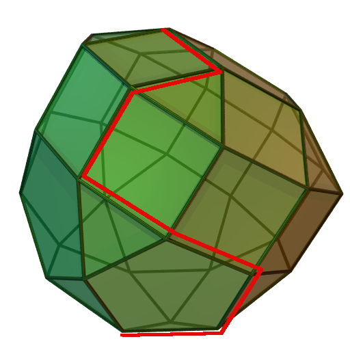
A linear programming polytope with a possible path (red) that the simplex method could take along its edges to solve the corresponding problem. User:Sdo, via Wikimedia Commons, CC BY-SA 3.0.
## Definition and standard forms
A general linear program in the notation of Boyd and Vandenberghe's *Convex Optimization* is:[3]
$$
\begin{aligned}
\text{minimize} \quad & c^T x + d \\
\text{subject to} \quad & Gx \preceq h \\
& Ax = b
\end{aligned}
$$
Here $x \in \mathbb{R}^n$ is the vector of decision variables, $c^T x + d$ is the objective, $G \in \mathbb{R}^{m \times n}$ and $h$ define the inequality constraints (the symbol $\preceq$ means componentwise $\le$), and $A \in \mathbb{R}^{p \times n}$ and $b$ define the equality constraints.[3] The constant $d$ is usually dropped because it does not change the optimal point, and a maximization problem with linear objective and constraints is also called an LP, since maximizing $c^T x$ is the same as minimizing $-c^T x$.[3]
Two special cases have their own names:[3]
| Form | Problem | Constraints |
|---|---|---|
| Standard form | minimize $c^T x$ | $Ax = b$, $x \succeq 0$ |
| Inequality form | minimize $c^T x$ | $Ax \preceq b$ |
Any general LP can be rewritten in standard form. Each inequality gets a nonnegative slack variable $s_i$ that turns it into an equality, and each unrestricted variable is split into the difference of two nonnegative variables, $x = x^+ - x^-$.[3] Problems that are not linear on their face can often be reformulated as LPs; for example, minimizing a convex piecewise-linear function $\max_i (a_i^T x + b_i)$ becomes an LP once an extra variable $t$ is introduced with the constraints $a_i^T x + b_i \le t$.[3]
Geometrically, the level sets of a linear objective are parallel [hyperplanes](https://aiwiki.ai/wiki/hyperplane), and the optimal solution is the point of the feasible polyhedron that lies as far as possible in the direction $-c$.[3] Dantzig's simplex method exploits this picture by moving along the edges of the polyhedron from one extreme point (vertex) to a neighbouring one until it reaches an optimal vertex.[2][9]
### A small example
Consider the problem of maximizing $3x_1 + 2x_2$ subject to $x_1 + x_2 \le 4$, $2x_1 + x_2 \le 6$, $x_1 \ge 0$ and $x_2 \ge 0$. The feasible region is a quadrilateral with vertices $(0,0)$, $(3,0)$, $(2,2)$ and $(0,4)$, where the objective takes the values 0, 9, 10 and 8. The optimum is therefore $x = (2, 2)$ with objective value 10. The same example is used below to illustrate duality.
"Optimization with Linear Programming (and the Simplex Algorithm), Main Ideas!!!", video from StatQuest with Josh Starmer, published July 6, 2026. Watch on YouTube.
## History
### Precursors
Dantzig himself noted that a few isolated authors had written about the problem before him: Joseph Fourier in 1823 and Charles de la Vallée Poussin in 1911, as well as Frank Hitchcock, whose 1941 paper treated the transportation problem.[1] He judged that the papers of Fourier and de la Vallée Poussin had essentially no influence on what came after 1947, and that Hitchcock's paper was overlooked until others had independently rediscovered its results.[1] Fourier devised an elimination procedure for systems of linear inequalities, now usually called Fourier-Motzkin elimination, which can in principle solve linear programs.[8] Richard Cottle's memoir of Dantzig points to an even earlier case: a method published in Latin in 1757 by Roger Joseph Boscovich and Christopher Maire for a least absolute value regression problem is equivalent to a variant of the simplex method.[2]
### Kantorovich, 1939
In 1938 Leonid Kantorovich, then a professor at Leningrad University, consulted for the laboratory of the Plywood Trust on a problem of distributing raw materials so as to maximize equipment productivity under restrictions. In his own words, mathematically it was "a problem of maximizing a linear function on a convex polytope".[4] He found that many other economic problems had the same form, among them assigning work to machines, using sowing area, cutting material and routing transport flows, and he developed a solution technique he called the "method of resolving multipliers".[4] His booklet *The Mathematical Method of Production Planning and Organization*, printed by Leningrad University Press in 1939, contained in his description "the main ideas of the theories and algorithms of linear programming".[4]
Dantzig wrote that Kantorovich's monograph "was also neglected for ideological reasons in the USSR" and was revived only about two decades later, after the main developments had taken place in the West.[1] On the initiative of Tjalling Koopmans, an English translation appeared in *Management Science* in 1960.[4][7] Kantorovich wrote that he learned of the parallel Western work of Koopmans, Dantzig and others only in the mid-1950s.[4]
### Koopmans and the transportation problem
In August 1942 the economist Tjalling Koopmans, then working on Allied wartime shipping, studied optimal routing and the associated "shadow costs" of transportation on different routes, expressed in ship days; his memorandum was well received at a meeting of the Combined Shipping Adjustment Board.[1][6] He later wrote that this work broadened into the study of activity analysis at the Cowles Commission after a conversation with George Dantzig, "probably in early 1947".[6]
### Dantzig and the simplex method, 1947
After finishing his PhD at Berkeley in 1946, Dantzig returned to the Pentagon as mathematical advisor to the comptroller of the newly created U.S. Air Force.[2] His Pentagon colleagues challenged him to mechanize the planning process, that is, to find a faster way to compute a time-staged program of deployment, training and logistical supply.[1] Dantzig admired Wassily Leontief's input-output model of the economy but needed a dynamic version with alternative activities.[1] By mid-1947 he had a model with an explicit linear objective function in place of the ad hoc "ground rules" planners had used to choose among feasible plans; he called the use of a linear objective "a novel feature of the model".[1]
In June 1947 Dantzig visited Koopmans at the Cowles Foundation in Chicago to see whether economists already had a solution method; they did not.[1] He proposed the simplex method in the summer of 1947, although, as he later wrote, it took nearly a year before he and his colleagues realized how powerful it was.[1] On October 3, 1947, he met John von Neumann at the Institute for Advanced Study in Princeton. Von Neumann, who had recently finished his book on the theory of games with Oskar Morgenstern, responded with a lecture of an hour and a half on the mathematical theory of linear programs.[1]
Dantzig originally titled his work "Programming in a Linear Structure", using "program" in the military sense of a plan or schedule.[1] In the summer of 1948, during a walk on the beach at Santa Monica, Koopmans suggested shortening the name to "linear programming", and Dantzig adopted it.[1][2] The name "simplex method" came from a discussion with Theodore Motzkin, who felt that Dantzig's approach, viewed in the geometry of the columns, was a movement from one simplex to a neighbouring one.[1] The word "primal", for the original problem paired with a dual, was proposed around 1954 by Dantzig's father, Tobias Dantzig.[1]
When Dantzig presented the model at a 1948 meeting of the Econometric Society at the University of Wisconsin, Harold Hotelling objected that "the world is nonlinear"; von Neumann answered on Dantzig's behalf that if an application satisfies the model's axioms it can be used, and otherwise not.[1][2] In 1949 Koopmans organized the first conference on the subject at the University of Chicago, whose proceedings were published as *Activity Analysis of Production and Allocation*.[1][2]
### Early computation
The first application of the simplex method to a non-trivial problem was a 21-constraint, 77-variable instance of George Stigler's diet problem, solved by Laderman in a computation reported to have taken 120 man-days.[10] The first computer implementation of a reasonably general simplex code ran on the SEAC computer at the National Bureau of Standards.[10] In 1952 Dantzig moved to the RAND Corporation, where he worked with William Orchard-Hays on a series of implementations: a 1953 version on a Card Programmable Calculator solved a 26-constraint, 71-variable Stigler model in about 8 hours, and a 1954-55 version on the IBM 701 handled 101 constraints.[10] Dantzig credited Orchard-Hays with writing, in 1954, "the first commercial-grade software for solving linear programs".[1] Commercial applications began in 1952 with work by Charnes, Cooper and Mellon on blending petroleum products into gasoline.[1]
### Recognition
The 1975 Sveriges Riksbank Prize in Economic Sciences in Memory of Alfred Nobel was awarded to Kantorovich and Koopmans "for their contributions to the theory of optimum allocation of resources".[5] Dantzig was not included, which Cottle describes as "a touch of controversy"; efforts by scholars to have his contribution recognized were unsuccessful.[2] In the same year Dantzig received the U.S. National Medal of Science and the John von Neumann Theory Prize.[2]
### Complexity: from Klee-Minty to Khachiyan
The simplex method usually performs well in practice, but in a paper published in 1972 Victor Klee and George Minty showed that in the worst case it can take a number of steps exponential in the size of the problem.[9] For a long time it was not known whether linear programs could be solved in polynomial time at all.[1] In 1979 Leonid Khachiyan showed that they can, using a modification of the ellipsoid method, an algorithm developed for nonlinear programming by N. Z. Shor, D. B. Yudin and A. S. Nemirovskii.[8][9] The New York Times reported the result on November 7, 1979, calling Khachiyan an "obscure Soviet mathematician".[8] The ellipsoid method proved to be impractical for computation, but it became a powerful theoretical tool for proving that many optimization problems, particularly in combinatorial optimization, can be solved in polynomial time.[8][10]
### Karmarkar and interior-point methods
In 1984 Narendra Karmarkar of Bell Labs published a polynomial-time algorithm based on projective transformations.[9][11] Its complexity bound was much better than Khachiyan's, and unlike the ellipsoid method it could be used in practice.[1][10] Karmarkar, supported by Bell Labs, claimed that an implementation of the method was vastly superior to the simplex method; at the 1985 International Symposium on Mathematical Programming in Boston, Karmarkar said his algorithm would be 50 or 100 times faster than the best simplex codes, a claim many in the audience received with skepticism.[9]
At the same meeting Margaret Wright presented work by P. Gill and co-authors showing that Karmarkar's method is a special case of the logarithmic barrier method developed by Anthony Fiacco and Garth McCormick in their 1968 book.[9] Barrier ideas went back further still: Ragnar Frisch had suggested a logarithmic potential method in an unpublished 1955 manuscript, and Dikin had published the affine scaling method in 1967.[9] AT&T obtained a U.S. patent on Karmarkar's method, filed in April 1985 and granted on May 10, 1988, and marketed a package called KORBX that combined an eight-processor computer with an interior-point code.[9][12] The patent caused a stir because mathematics had until then been considered unpatentable.[9] David Shanno, who co-developed the OB1 primal-dual interior-point code, later wrote that, according to KORBX team member Robert Vanderbei, KORBX actually implemented the affine scaling method rather than the patented projective algorithm.[9] KORBX was largely unsuccessful commercially, but primal-dual log-barrier algorithms became the standard interior-point approach, and commercial codes such as CPLEX added barrier solvers alongside primal and dual simplex.[9][10]
### Later theoretical results
In 2001 Daniel Spielman and Shang-Hua Teng introduced smoothed analysis, which measures an algorithm's worst-case expected performance when its input is slightly perturbed at random, and showed that the simplex method has polynomial smoothed complexity.[13] Their original bound was later improved in a series of papers; in 2025 Eleon Bach and Sophie Huiberts proved an upper bound for a simplex method together with a lower bound showing its dependence on the noise level is optimal among all simplex methods, up to polylogarithmic factors.[14]
A related geometric question is the Hirsch conjecture, which Dantzig recorded in his 1963 book *Linear Programming and Extensions* and credited to Warren Hirsch. In modern terms it states that the graph of a $d$-dimensional polyhedron with $n$ facets has diameter at most $n - d$; Hirsch and Dantzig were interested in it as a bound on the number of pivot steps the simplex method might need.[15] Victor Klee and David Walkup disproved the version for unbounded polyhedra in 1967, and in 2010 Francisco Santos disproved the bounded version with a 43-dimensional polytope with 86 facets and diameter greater than 43.[15] Writing in 2012, Günter Ziegler noted that the best known upper bounds on polytope diameters were still only mildly sub-exponential, so whether a good (for example, linear) bound holds remained unknown.[15]
On the interior-point side, Michael Cohen, Yin Tat Lee and Zhao Song showed in a paper presented at STOC 2019 that an LP $\min\{c^T x : Ax = b, x \ge 0\}$ with $n$ variables can be solved in time $O^*(n^{\omega} \log(n/\delta))$ for the current value of $\omega$ (about 2.37), where $\omega$ is the exponent of matrix multiplication and $\delta$ the relative accuracy.[16]
## Duality
Every linear program has a dual linear program. For a standard form LP, the Lagrange dual problem can be written as:[3]
$$
\begin{aligned}
\text{maximize} \quad & -b^T \nu \\
\text{subject to} \quad & A^T \nu + c \succeq 0
\end{aligned}
$$
which is itself an LP in inequality form.[3] For a minimization problem, weak duality says that the dual optimal value is a lower bound on the primal optimal value. Strong duality, equality of the two values, holds for any LP whose primal or dual problem is feasible; the only case in which it fails is when both are infeasible.[3] At an optimal pair of primal and dual solutions, complementary slackness holds: an optimal dual variable can be nonzero only if its constraint is active (holds with equality) at the optimum.[3] When the optimal value is differentiable in the constraint data, the optimal dual variables are its local sensitivities: they say how much the optimal value changes when a constraint is loosened or tightened slightly, which is why they are often read as prices.[3]
In the example above, the dual problem is to minimize $4y_1 + 6y_2$ subject to $y_1 + 2y_2 \ge 3$, $y_1 + y_2 \ge 2$ and $y_1, y_2 \ge 0$. Its optimum is $y = (1, 1)$ with value 10, equal to the primal optimum. Both primal constraints are tight at $x = (2, 2)$, consistent with both dual variables being positive, and raising either right-hand side by one unit raises the primal optimum by one.
Dantzig's account traces duality theory to his 1947 conversation with von Neumann, who presented it as an analogue of the theory he and Morgenstern had developed for [games](https://aiwiki.ai/wiki/game_theory) and conjectured that the two problems were equivalent.[1] Dantzig wrote that this meeting was where he first learned of Farkas' lemma and of duality.[1]
## Algorithms
| Method | Introduced | How it moves | Notes |
|---|---|---|---|
| Simplex method | Dantzig, 1947 | Along edges between vertices of the feasible polyhedron | Exponential worst case (Klee-Minty, 1972) but fast in practice; polynomial smoothed complexity[1][9][13] |
| Dual simplex method | C. E. Lemke, 1954 | Simplex steps on the dual problem | Long used mainly for re-optimization in branch-and-bound; a general-purpose solver from the early 1990s[10] |
| Ellipsoid method | Khachiyan, 1979 | Shrinking ellipsoids that contain the solution set | First polynomial-time LP algorithm; not practical[8][10] |
| Projective interior-point method | Karmarkar, 1984 | Through the interior of the polyhedron | Polynomial bound; began the interior-point era[9][10] |
| Primal-dual barrier methods | Late 1980s | Newton steps on the optimality conditions of a logarithmic barrier problem | Standard interior-point approach; parallelize well[9][10] |
| First-order methods (PDHG, PDLP) | 2021 (PDLP) | Matrix-vector products on a saddle-point form | Scale to very large problems and run on GPUs[17][18] |
### Simplex and barrier in practice
Robert Bixby measured the progress of the CPLEX LP code between 1988 and 2004 and found that algorithmic improvements alone, independent of hardware, sped it up by a factor of roughly 3,300; combined with faster computers the total exceeded six orders of magnitude.[10] He reported that by 2012 primal simplex was rarely the fastest choice. The dual simplex method and barrier methods dominated, and barrier methods were increasingly winning on large problems because they can be parallelized, while there had been essentially no success in parallelizing simplex.[10] Barrier solutions are usually followed by a "crossover" step to a vertex (basic) solution, which is needed for warm starts in integer programming.[10] Bixby also noted a common view among practitioners that LP is a "solved problem", with problems of several hundred thousand constraints and variables solved routinely, while warning that the difficulty of the underlying LPs still blocked the solution of roughly 2 percent of real-world mixed-integer models.[10]
### First-order and GPU methods
A newer line of work applies first-order methods. PDLP, described by David Applegate and colleagues at NeurIPS 2021, applies the primal-dual hybrid gradient (PDHG) method to a saddle-point formulation of LP; its core operation is matrix-vector multiplication, which lets it scale to very large problems.[17] In 2023 Haihao Lu and Jinwen Yang released cuPDLP.jl, a GPU implementation in Julia, and reported performance comparable to the commercial Gurobi solver on standard LP benchmark sets.[18] In March 2025 [NVIDIA](https://aiwiki.ai/wiki/nvidia) announced that it would open-source its cuOpt optimization engine in partnership with the COIN-OR Foundation, claiming GPU LP speedups averaging 70 times over a CPU-based PDLP solver on large benchmarks.[19] As of November 2026 the cuOpt repository is published under the Apache 2.0 licence and lists LP, quadratic programming and vehicle routing as its main problem types, with mixed-integer, quadratically constrained and second-order cone programming in beta.[20] Commercial solvers have adopted the same approach: Gurobi 13.0, released on November 18, 2025, added a PDHG implementation for some large-scale LPs, with CPU and GPU support.[30]
### Software
Commercial LP solvers run from Orchard-Hays's RAND codes through IBM's MPSX to CPLEX (first released in 1988), IBM's OSL, Xpress and Gurobi, whose first release came in 2009.[10] Open-source options include HiGHS, an MIT-licensed linear optimization library.[21] HiGHS is the default method of the [SciPy](https://aiwiki.ai/wiki/scipy) function `scipy.optimize.linprog`, which can also call its dual simplex and interior-point solvers directly.[22]
## Integer and mixed-integer programming
Integer programming adds the requirement that some or all variables take integer values, such as 0-1 variables that record yes-or-no decisions; a model mixing integer and continuous variables is a mixed-integer program (MIP).[1][10] Bixby wrote that while LP is fundamental, in practical optimization "it is MIP that dominates".[10] MIP solvers are built on top of LP solvers. Branch-and-bound search solves a sequence of linear programs while it explores a tree of restrictions on the integer variables; the first commercially used branch-and-bound MIP code was a conversion of the LP/90/94 system begun around 1964-65 by Beale and Small, using an approach suggested by Land and Doig.[10] Cutting planes, extra linear inequalities that every integer solution must satisfy, have roots in the 1954 traveling salesman work of Dantzig, D. R. Fulkerson and S. M. Johnson, and R. E. Gomory showed in 1958 how to generate them systematically.[1][10] Bixby described a jump in 1998, when CPLEX 6.5 systematically incorporated decades of such research and became more than ten times faster than its predecessor on his test set.[10]
## Applications in operations research
Linear programming began in military logistics, and commercial applications soon eclipsed the military ones.[1] By the late 1950s it was beginning to see significant use in the oil industry.[10] Classic applications include:
| Application | Typical question | Sources |
|---|---|---|
| Diet problem | Cheapest combination of foods that meets nutritional requirements; the model of the first large simplex computations | [3][10] |
| Transportation and network flow | Least-cost shipment of goods from suppliers to consumers; developed in the 1950s into network flow theory | [1][4][6] |
| Assignment | Best assignment of people to jobs | [1] |
| Production planning and blending | Allocating raw materials and machines, blending petroleum products | [1][4] |
| Scheduling, financial planning, marketing | Best activity levels for an objective under resource limits | [2] |
Dantzig used the assignment problem to show why algorithms matter: assigning 70 people to 70 jobs has 70! possible solutions, a number greater than $10^{100}$, far too many to compare by brute force, yet standard simplex or interior-point software finds the optimum in a moment on a personal computer.[1] Linear programs also arise as subproblems inside algorithms for nonlinear optimization.[2]
## Linear programming in machine learning and AI
### Fitting and estimation
Several estimation problems are LPs. Minimizing the sum of absolute residuals $\|Ax - b\|_1$, the problem behind least-absolute-deviation regression and the [mean absolute error](https://aiwiki.ai/wiki/mean_absolute_error_mae) loss, can be cast as an LP with one auxiliary variable per data point; Boyd and Vandenberghe describe it as a robust estimator.[3] Chebyshev (minimax) approximation, which minimizes the largest residual, is also an LP.[3] In signal processing, basis pursuit, introduced by Scott Chen, David Donoho and Michael Saunders, decomposes a signal into a dictionary of waveforms by minimizing the $\ell_1$ norm of the coefficients; the problem is equivalent to a linear program, and the authors relied on interior-point methods to solve instances with hundreds of thousands of variables. In their examples it gave sparser representations than competing methods such as matching pursuit.[23] Sparse representation is also the aim of [sparse coding](https://aiwiki.ai/wiki/sparse_coding).
### Optimal transport and the Earth mover's distance
The [Earth mover's distance](https://aiwiki.ai/wiki/earth_mover_s_distance), proposed for image retrieval by Yossi Rubner, Carlo Tomasi and Leonidas Guibas, is the minimal cost of turning one distribution into another. Computing it means solving the transportation problem, which the authors formalize as a linear program, citing Hitchcock's 1941 paper, and solve with the transportation-simplex method, a simplex variant that exploits the problem's special structure.[24]
### Approximate dynamic programming
Exact dynamic programming becomes infeasible for large stochastic control problems because of the curse of dimensionality. Daniela Pucci de Farias and Benjamin Van Roy studied a linear programming method for approximating solutions to such problems: it fits a linear combination of preselected basis functions to the dynamic programming cost-to-go function (the [value function](https://aiwiki.ai/wiki/value_function)) by solving an LP. They derived error bounds that guarantee performance and guide the choice of basis functions, and tested the method on queueing network control.[25]
### Robustness and verification of neural networks
Linear programming has been used to certify neural networks against [adversarial attacks](https://aiwiki.ai/wiki/adversarial_attack). Eric Wong and J. Zico Kolter proposed a method, presented at ICML, that replaces the set of [ReLU](https://aiwiki.ai/wiki/relu) network activations reachable under a norm-bounded input perturbation with a convex outer approximation and bounds the worst-case loss over it by solving a linear program. They showed that the dual of this LP can itself be represented as a deep network similar to the backpropagation network, so that robust training needs only a few extra forward and backward passes through a modified version of the original network.[26]
### Learning inside solvers
Machine learning is also used to speed up solvers. Maxime Gasse and co-authors represented mixed-integer linear programs as bipartite graphs of variables and constraints and trained a [graph neural network](https://aiwiki.ai/wiki/graph_neural_network) by [imitation learning](https://aiwiki.ai/wiki/imitation_learning) to choose branching variables in branch-and-bound; at NeurIPS 2019 they reported improving on the expert-designed branching rule of a state-of-the-art solver on large problems.[27]
### Language models that formulate LPs
Writing an LP model from a verbal description takes expertise, and recent work tests whether language models can do it.[28][29] The NL4Opt competition at NeurIPS 2022 released a dataset of linear programming word problems and asked participants to extract the elements of the optimization problem and generate a formulation that solvers can use.[28] OptiMUS, an agent built on a large language model by Ali AhmadiTeshnizi, Wenzhi Gao and Madeleine Udell, formulates and solves mixed-integer linear programs from natural language, writes and debugs solver code, and was evaluated on a new dataset of LP and MILP problems called NLP4LP; the authors reported that it solved nearly twice as many problems as a basic prompting strategy.[29]
## See also
- [Convex optimization](https://aiwiki.ai/wiki/convex_optimization)
- [Convex set](https://aiwiki.ai/wiki/convex_set)
- [Dynamic programming](https://aiwiki.ai/wiki/dynamic_programming)
- [Earth mover's distance](https://aiwiki.ai/wiki/earth_mover_s_distance)
- [Nash equilibrium](https://aiwiki.ai/wiki/nash_equilibrium)
## References
1. Dantzig, George B. "Linear Programming". Operations Research, vol. 50, no. 1, January-February 2002, pp. 42-47. https://doi.org/10.1287/opre.50.1.42.17798
2. Cottle, Richard W. "George B. Dantzig, November 8, 1914-May 13, 2005". Biographical Memoirs, National Academy of Sciences, 2024. https://www.nasonline.org/wp-content/uploads/2024/06/dantzig-george-b.pdf
3. Boyd, Stephen; Vandenberghe, Lieven. "Convex Optimization". Cambridge University Press, 2004 (sections 4.3, 5.2, 5.5 and 6.1). https://web.stanford.edu/~boyd/cvxbook/bv_cvxbook.pdf
4. Kantorovich, Leonid V. "Leonid Vitaliyevich Kantorovich - Biographical". NobelPrize.org. https://www.nobelprize.org/prizes/economic-sciences/1975/kantorovich/biographical/
5. NobelPrize.org. "The Sveriges Riksbank Prize in Economic Sciences in Memory of Alfred Nobel 1975". https://www.nobelprize.org/prizes/economic-sciences/1975/summary/
6. Koopmans, Tjalling C. "Tjalling C. Koopmans - Biographical". NobelPrize.org. https://www.nobelprize.org/prizes/economic-sciences/1975/koopmans/biographical/
7. Kantorovich, L. V. "Mathematical Methods of Organizing and Planning Production". Management Science, vol. 6, no. 4, July 1960, pp. 366-422. https://doi.org/10.1287/mnsc.6.4.366
8. Grötschel, Martin. "Linear Programming Stories". Documenta Mathematica, Extra Volume: Optimization Stories (ISMP 2012), pp. 51-53. https://www.maths.tcd.ie/EMIS/journals/DMJDMV/vol-ismp/20_Linear-programming-stories.pdf
9. Shanno, David. "Who Invented the Interior-Point Method?". Documenta Mathematica, Extra Volume: Optimization Stories (ISMP 2012), pp. 55-64. https://www.maths.tcd.ie/EMIS/journals/DMJDMV/vol-ismp/20_shanno-david.pdf
10. Bixby, Robert E. "A Brief History of Linear and Mixed-Integer Programming Computation". Documenta Mathematica, Extra Volume: Optimization Stories (ISMP 2012), pp. 107-121. https://www.maths.tcd.ie/EMIS/journals/DMJDMV/vol-ismp/25_bixby-robert.pdf
11. Karmarkar, N. "A new polynomial-time algorithm for linear programming". Combinatorica, vol. 4, no. 4, 1984, pp. 373-395. https://doi.org/10.1007/BF02579150
12. Karmarkar, Narendra K. (AT&T Bell Laboratories). "Methods and apparatus for efficient resource allocation". U.S. Patent 4,744,028, granted May 10, 1988. https://patents.google.com/patent/US4744028A/en
13. Spielman, Daniel A.; Teng, Shang-Hua. "Smoothed Analysis of Algorithms: Why the Simplex Algorithm Usually Takes Polynomial Time". arXiv:cs/0111050, 2001. https://arxiv.org/abs/cs/0111050
14. Bach, Eleon; Huiberts, Sophie. "Optimal Smoothed Analysis of the Simplex Method". arXiv:2504.04197, 2025. https://arxiv.org/abs/2504.04197
15. Ziegler, Günter M. "Who Solved the Hirsch Conjecture?". Documenta Mathematica, Extra Volume: Optimization Stories (ISMP 2012), pp. 75-85. https://www.maths.tcd.ie/EMIS/journals/DMJDMV/vol-ismp/22_ziegler-guenter.pdf
16. Cohen, Michael B.; Lee, Yin Tat; Song, Zhao. "Solving Linear Programs in the Current Matrix Multiplication Time". arXiv:1810.07896 (STOC 2019), 2018. https://arxiv.org/abs/1810.07896
17. Applegate, David; Díaz, Mateo; Hinder, Oliver; Lu, Haihao; Lubin, Miles; O'Donoghue, Brendan; Schudy, Warren. "Practical Large-Scale Linear Programming using Primal-Dual Hybrid Gradient". arXiv:2106.04756 (NeurIPS 2021), 2021. https://arxiv.org/abs/2106.04756
18. Lu, Haihao; Yang, Jinwen. "cuPDLP.jl: A GPU Implementation of Restarted Primal-Dual Hybrid Gradient for Linear Programming in Julia". arXiv:2311.12180, 2023. https://arxiv.org/abs/2311.12180
19. Neskovic, Gordana. "NVIDIA Open-Sources cuOpt, Ushering in New Era of Decision Optimization". NVIDIA Blog, March 18, 2025. https://blogs.nvidia.com/blog/cuopt-open-source/
20. NVIDIA. "cuOpt - GPU-accelerated Optimization" (repository README). GitHub, accessed November 2026. https://github.com/NVIDIA/cuopt
21. ERGO-Code. "HiGHS: Linear optimization software" (repository). GitHub, accessed November 2026. https://github.com/ERGO-Code/HiGHS
22. SciPy. "scipy.optimize.linprog". SciPy v1.18.0 Manual. https://docs.scipy.org/doc/scipy/reference/generated/scipy.optimize.linprog.html
23. Chen, Scott Shaobing; Donoho, David L.; Saunders, Michael A. "Atomic Decomposition by Basis Pursuit". SIAM Review, vol. 43, no. 1, 2001, pp. 129-159 (originally SIAM Journal on Scientific Computing, 1998). https://web.stanford.edu/group/SOL/papers/BasisPursuit-SIGEST.pdf
24. Rubner, Yossi; Tomasi, Carlo; Guibas, Leonidas J. "The Earth Mover's Distance as a Metric for Image Retrieval". International Journal of Computer Vision, vol. 40, no. 2, 2000, pp. 99-121. https://doi.org/10.1023/A:1026543900054
25. de Farias, D. P.; Van Roy, B. "The Linear Programming Approach to Approximate Dynamic Programming". Operations Research, vol. 51, no. 6, 2003, pp. 850-865. https://doi.org/10.1287/opre.51.6.850.24925
26. Wong, Eric; Kolter, J. Zico. "Provable defenses against adversarial examples via the convex outer adversarial polytope". arXiv:1711.00851, 2017 (ICML 2018). https://arxiv.org/abs/1711.00851
27. Gasse, Maxime; Chételat, Didier; Ferroni, Nicola; Charlin, Laurent; Lodi, Andrea. "Exact Combinatorial Optimization with Graph Convolutional Neural Networks". arXiv:1906.01629 (NeurIPS 2019), 2019. https://arxiv.org/abs/1906.01629
28. Ramamonjison, Rindranirina; et al. "NL4Opt Competition: Formulating Optimization Problems Based on Their Natural Language Descriptions". arXiv:2303.08233, 2023. https://arxiv.org/abs/2303.08233
29. AhmadiTeshnizi, Ali; Gao, Wenzhi; Udell, Madeleine. "OptiMUS: Optimization Modeling Using MIP Solvers and large language models". arXiv:2310.06116, 2023. https://arxiv.org/abs/2310.06116
30. Gurobi Optimization. "Gurobi Releases Version 13.0 with Improved Performance and New Solving Capabilities". Gurobi newsroom, November 18, 2025. https://www.gurobi.com/company/newsroom/gurobi-releases-version-13-0-with-improved-performance-and-new-solving-capabilities