Diffusion Models
Diffusion Models (DMs) are generative models, meaning they are designed to generate data resembling the training data. They have gained significant attention in recent years due to their ability to outperform other generative models, such as Generative Adversarial Networks (GANs). [1][2][3]These models were notably employed in OpenAI's DALL-E 2, an image generation model[1]. Generative models, including Diffusion Models, GANs, Variational Autoencoders (VAEs), and Flow-based models, are designed to generate data resembling the training data. [1][3]
Diffusion Models have surpassed GANs' dominance in image synthesis and demonstrated potential across various domains, including computer vision, natural language processing, temporal data modeling, multi-modal modeling, robust machine learning, and interdisciplinary applications such as computational chemistry and medical image reconstruction. [4]
How do Diffusion Models work?
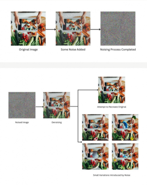
Diffusion Models operate in two main phases: the forward diffusion process and the reverse diffusion process. In the forward diffusion process, the model progressively corrupts the training data by adding Gaussian noise in a series of steps, referred to as the "noise schedule". The reverse diffusion process involves learning to denoise the corrupted data, ultimately recovering the original data (figure 1). [4] After training, the Diffusion Model can generate new data by passing randomly sampled noise through the learned denoising process. [1]
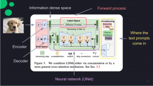
In a text-to-image model, the original image, represented by x, is fed into an encoder and encoded into Z, an information-dense space (figure 2). The forward process involves performing diffusion and conditioning with text, which combines text embeddings with the processed image. The merged inputs then become part of the initial noise for the diffusion process and pass through a UNet, a type of convolutional neural network, that predicts the noise in an image. The noise is then reconstructed through the decoder, resulting in the desired image. [4]
Therefore, the main components of this architecture are[2]:
- The forward process.
- The neural network.
- The conditioning aspect.
However, diffusion models have some drawbacks, such as a large number of sampling steps, long sampling time, and difficulties with likelihood optimization and dimension reduction. [3]
Forward Process and Markov Chain
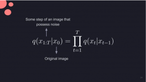
Diffusion models destroy input data by gradually adding noise through a forward process that can be executed using Markov Chains (figure 3). In the case of a particular image, x₀, a noisy image can be created by adding a sequence of Gaussian noise. [4] A diffusion model is a latent variable model that maps to the latent space using a fixed Markov chain. This chain gradually adds noise to the data to obtain the approximate posterior q(x1:T|x0), where x1,..., xT are the latent variables with the same dimensionality as x0 (figure 4). [5]
Gaussian Noise and Beta
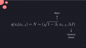
The sequence of betas is named variance schedule, describing how much noise is added at each timestep. [4] The image is transformed into pure Gaussian noise asymptotically, and the goal of training a diffusion model is to learn the reverse process by training p0(xt-1|xt). [5] For a pixel with three channels (R, G, and B), a specific channel (e.g., green) has the equation in figure 5 applied to it. The Beta value influences how the pixel distribution and normal curve are affected. A larger Beta value results in a wider pixel distribution and a normal curve shifted further towards 0. The image corruption increases as it strays further from the original. [4]
Noise Scheduling and Neural Network
A noise schedule is a sequence of Beta values applied at each timestep (t) to add the right amount of noise, so that an isotropic Gaussian distribution with a mean of 0 and fixed variance in all directions is achieved. This allows the denoising process to function effectively. [4] The neural network is used to reverse the process and predict images with just noise. It acts as a denoising mechanism, removing the "impurities" of the image gradually until it recovers or generates a high-quality image[4]. The pairs of images and captions used to train the neural network are from the LAION-5B dataset. [4]
Conditioning
In the conditioning step, a text prompt is added to the noisy image—for example, "a smiley face." The image passes through the neural network and predicts the noise again, but with the associated latent space representation of a smiley face acquired through training. The neural network incorporates the noise created by a smiley face into the prediction. [4]
Importance of Diffusion Models
Diffusion models, representing the apex of generative capabilities, owe their success to advancements in machine learning techniques, abundant image data, and improved hardware. Distinguished from predecessors like GANs, diffusion models generate highly realistic images and offer better stability, avoiding issues like mode collapse, thus providing more diverse imagery. [2]
These models can be conditioned on different inputs and have numerous evolving applications, with potential to impact industries such as retail and eCommerce, entertainment, social media, AR/VR, and marketing. [2]
Prompts
In DMs, controlling outputs is achieved through prompts. These models require two main inputs, a seed integer and a text prompt, which are then translated into a fixed point within the model's latent space. While the seed integer is typically auto-generated, the user supplies the text prompt. Engaging in experimentation through prompt engineering is essential for obtaining optimal results. [2]
Diffusion Model Formulations
Diffusion models are built upon three main formulations: denoising diffusion probabilistic models (DDPMs), score-based generative models (SGMs), and stochastic differential equations (Score SDEs). These three models work under the same principle of diffusion, progressively perturbing data with increasing random noise and then successively removing noise to generate new data samples. [3]
These models gained popularity due to their stable training compared to GANs and the higher quality of generated samples. Some limitations of GANs are addressed by DMs, such as mode collapse, adversarial learning overhead, and convergence failure. Their training process differs significantly from GANs, as it involves perturbing training data with Gaussian noise and then learning to recover the original data from the noisy version. [6] The concept of diffusion models is illustrated in figure 6, and current research primarily focuses on the aforementioned formulations. [3]
Denoising Diffusion Probabilistic Models (DDPMs) utilize two Markov chains: one that transforms data into noise, and another that converts noise back into data. The first chain is designed to convert any data distribution into a simpler prior distribution, such as a standard Gaussian, while the second chain reverses this process by learning transition kernels using deep neural networks. [3]
Score-Based Generative Models (SGMs) rely on the concept of (Stein) score, also known as score or score function. The fundamental idea these models is to disturb data with intensifying Gaussian noise while simultaneously estimating “score functions for all noisy data distributions by training a deep neural network model conditioned on noise levels,” called a noise-conditional score network (NCSN). According to Yang, et al. (2023), “samples are generated by chaining score functions at decreasing noise levels” using various score-based sampling approaches, such as Langevin Monte Carlo, stochastic differential equations, ordinary differential equations, and their combinations. In SGMs, training and sampling are completely decoupled, allowing for multiple sampling techniques after estimating score functions. [3]
Yang et al. (2023) also mentions that Stochastic Differential Equations (Score SDEs) generalize DDPMs and SGMs “to the case of infinite time steps or noise levels,” with perturbation and denoising processes serving as solutions to stochastic differential equations (SDEs). This formulation, called Score SDE, leverages SDEs for noise perturbation and sample generation, requiring the estimation of score functions for noisy data distributions in the denoising process. [3]
Applications of Diffusion Models
Figure 7. Applications using diffusion models. Source: Yang et al. (2023)
Research has increased for diffusion models. These produce state-of-the-art image quality and ability to generate a diverse range of images from text alone. [1][2] These models offer numerous advantages, such as not requiring adversarial training, scalability, and parallelizability. [1] They can perform various tasks, including image generation, denoising, inpainting, outpainting, and bit diffusion. [2]
The potential applications of diffusion models are vast (figure 7), spanning across industries such as retail and eCommerce, product design, marketing, entertainment, and augmented and virtual reality. By integrating diffusion models into design tools and other technologies, professionals can enhance creativity, efficiency, and explore new possibilities in their respective fields. For instance, diffusion models can be used to dynamically generate ad creatives, improve special effects in movies, and allow users to alter their virtual environments in real-time. [2]
In their research paper, “Diffusion Models: A Comprehensive Survey of Methods and Applications,” Yang et al. (2023) grouped the applications of DMs into six categories based on the task:
- Computer vision.
- Natural language processing.
- Temporal data modeling.
- Multi-modal learning.
- Robust learning.
- Interdisciplinary applications.
Limitations
Despite their potential, diffusion models also possess certain limitations. First, faces become distorted, as when the number of subjects in an image exceeds three. Additionally, these models struggle to generate text within images, despite being proficient at handling text prompts for image generation. Furthermore, achieving desired outputs may require extensive manipulation of prompts, which could reduce their efficiency as productivity tools, although they still contribute positively to productivity overall. [2]
References
- ↑ Jump up to: 1.0 1.1 1.2 1.3 1.4 O'Connor, R (2022). Introduction to Diffusion Models for Machine Learning. AssemblyAI. https://www.assemblyai.com/blog/diffusion-models-for-machine-learning-introduction/
- ↑ Jump up to: 2.0 2.1 2.2 2.3 2.4 2.5 2.6 2.7 2.8 Muppalla, V and Hendryx, S (2022). Diffusion Models: A Practical Guide. Scale. https://scale.com/guides/diffusion-models-guide
- ↑ Jump up to: 3.0 3.1 3.2 3.3 3.4 3.5 3.6 3.7 Yang, L, Zhang, Z, Song, Y, Hong, S, Xu, R, Zhao, Y, Zhang, W, Cui, B and Yang, M-H (2023). Diffusion Models: A Comprehensive Survey of Methods and Applications. arXiv:2209.00796v10. https://arxiv.org/pdf/2209.00796.pdf
- ↑ Jump up to: 4.0 4.1 4.2 4.3 4.4 4.5 4.6 4.7 4.8 Wei, YC (2022). Beginner's Guide to Diffusion Models. Towards Data Science. https://towardsdatascience.com/beginners-guide-to-diffusion-models-8c3435ccb4ae
- ↑ Jump up to: 5.0 5.1 O'Connor, R (2022). Introduction to Diffusion Models for Machine Learning. AssemblyAI. https://www.assemblyai.com/blog/diffusion-models-for-machine-learning-introduction/
- ↑ Ulhaq, A, Akhtar, N and Pogrebna, G (2022). Efficient Diffusion Models for Vision: A Survey. arXiv:2210.09292v2. https://arxiv.org/pdf/2210.09292.pdf
