Neural network: Difference between revisions
No edit summary |
m (Text replacement - "Category:Machine learning terms" to "Category:Machine learning terms Category:not updated") |
||
| (One intermediate revision by the same user not shown) | |||
| Line 10: | Line 10: | ||
The nodes (a place where computation happens) are organized in layers. They combine input from the data with weights (or coefficients), as mentioned above, amplifying or dampening the input, and consequently assigning significance to inputs for the task the algorithm is trying to learn. The input weight products are then summed and the result is passed through a node’s activation function in order to determine if a signal progresses further through the network and, if so, to what extent. The pairing of adjustable weights with input features is how significance is assigned to those features with regard to how the network classifies and clusters input <ref name="”4”" />. | The nodes (a place where computation happens) are organized in layers. They combine input from the data with weights (or coefficients), as mentioned above, amplifying or dampening the input, and consequently assigning significance to inputs for the task the algorithm is trying to learn. The input weight products are then summed and the result is passed through a node’s activation function in order to determine if a signal progresses further through the network and, if so, to what extent. The pairing of adjustable weights with input features is how significance is assigned to those features with regard to how the network classifies and clusters input <ref name="”4”" />. | ||
A node layer is a row of the artificial neurons that turn on or off as the input passes through the net (figure 1). The output of each layer is the subsequent layer’s input. The process starts from an initial input layer that receives the data. The number of input and output nodes in an ANN depends on the problem to which the network is being applied. Conversely, there are no fixed rules as to how many nodes the hidden layer should have. If it has few nodes, the network might have difficulty generalizing to problems it has never encountered before; if there are too many nodes, the network may take a long time to learn anything of value <ref name="”4”" />. | A node layer is a row of the artificial neurons that turn on or off as the input passes through the net (figure 1). The output of each layer is the subsequent layer’s input. The process starts from an initial input layer that receives the data. The number of input and output nodes in an ANN depends on the problem to which the network is being applied. Conversely, there are no fixed rules as to how many nodes the [[hidden layer]] should have. If it has few nodes, the network might have difficulty generalizing to problems it has never encountered before; if there are too many nodes, the network may take a long time to learn anything of value <ref name="”4”" />. | ||
An efficient way to solve complex problems is to decompose the complex system into simpler elements to be able to understand it. On the other side, simple elements can be gathered to produce a complex system. The network structure is one approach to achieve this. Even though there are a number of different types of networks, they can be generalized as having the following components: a set of nodes and connections between them. These can be seen as the computational units, receiving inputs and processing them to obtain an output. The complexity of the processing can vary. It can be simple, like summing the inputs, or complex, in which a node might contain another network, for example. The interactions of the nodes through the connections between them lead to a global behavior of the network. This behavior cannot be observed in the single elements that form the network. This is called an emergent behavior, in which the abilities of the network as a whole supersede the ones of its constitutive elements <ref name="”6”" />. | An efficient way to solve complex problems is to decompose the complex system into simpler elements to be able to understand it. On the other side, simple elements can be gathered to produce a complex system. The network structure is one approach to achieve this. Even though there are a number of different types of networks, they can be generalized as having the following components: a set of nodes and connections between them. These can be seen as the computational units, receiving inputs and processing them to obtain an output. The complexity of the processing can vary. It can be simple, like summing the inputs, or complex, in which a node might contain another network, for example. The interactions of the nodes through the connections between them lead to a global behavior of the network. This behavior cannot be observed in the single elements that form the network. This is called an emergent behavior, in which the abilities of the network as a whole supersede the ones of its constitutive elements <ref name="”6”" />. | ||
| Line 83: | Line 83: | ||
==The backpropagation algorithm== | ==The backpropagation algorithm== | ||
The [[backpropagation]] algorithm is used in layered feedforward ANNs, and it is one of the most popular algorithms. The artificial neurons, organized in layers, send their signals “forward” and the errors are propagated backwards. This algorithm uses supervised learning, in which examples of the inputs and outputs that are intended for the network compute are provided. The error, which is the difference between actual and expected results, is then calculated. The goal of the backpropagation algorithm is to reduce the error, until the ANN learns the training data. The training begins with random weights, and the objective is to adjust them to achieve a minimal error level. Resuming, the backpropagation algorithm can be broken down to four main steps: 1) feedforward computation; 2) back propagation to the output layer; 3) back propagation to the hidden layer, and 4) weight updates <ref name="”6”" /> <ref name="”8”" />. | |||
==Explain Like I'm 5 (ELI5)== | |||
Neural networks are computer programs designed to mimic the human brain's workings. Just as our brain contains millions of tiny [[neuron]]s working together in synapses to facilitate thoughts and decision-making, a neural network contains many small components called [[artificial neuron]]s working together in order to solve problems. | |||
When we learn something new, like how to ride a bike, our brain changes the connections between neurons in order to retain what was learned. In a similar fashion, an artificial neural network can alter its artificial neurons' connections in order to learn from data and make better decisions. | |||
For instance, if we want the neural network to recognize photos of cats, then we must show it an extensive library of images of cats and explain what makes a cat a cat. After viewing enough [[examples]], even if it has never seen that particular breed before, the neural network should be able to accurately recognize a picture of a cat as one. | |||
Neural networks are like superhuman computer brains that learn and make decisions independently! | |||
==References== | ==References== | ||
<references /> | <references /> | ||
[[Category:Terms]] [[Category:Machine learning terms]] | [[Category:Terms]] [[Category:Machine learning terms]] [[Category:not updated]] | ||
Latest revision as of 20:25, 17 March 2023
- See also: Machine learning terms
Introduction
Neural networks are machine learning algorithms modeled after the structure and function of the human brain, designed to recognize patterns and make decisions based on input data. An artificial neural network (ANN), or just neural network (NN) for simplicity, is a massively parallel distributed processor made up of simple, interconnected processing units. It is an information processing paradigm – a computing system - inspired by biological nervous systems (e.g. the brain) and how they process information, where a large number of highly interconnected processing units work in unison to solve specific problems. The scale of an artificial neural network is smaller when compared to their biological counterpart. For example, a large ANN might have hundreds or thousands of processor units while a biological nervous system (e.g. a mammalian brain) has billions of neurons [1] [2] [3]. Neural networks - a set of algorithms designed to recognize patterns - interpret data, labeling or clustering raw input. They recognize numerical patterns contained in vectors, into which all real-world data, such as images, sound, text, or time series need to be translated [4].
The simple processing units of an ANN are, in loose terms, the artificial equivalent of their biological counterpart, the neurons. Biological neurons receive signals through synapses. When the signals are strong enough and surpass a certain threshold, the neuron is activated, emitting a signal through the axon that might be directed to another synapse [4] [5] [6]. According to Gershenson (2003), the nodes (artificial neurons) “consist of inputs (like synapses), which are multiplied by weights (strength of the respective signals), and then computed by a mathematical function which determines the activation of the neuron. Another function (which may be the identity) computes the output of the artificial neuron (sometimes in dependence of a certain threshold). ANNs combine artificial neurons in order to process information [6].”
Weights represent a factor by which values that pass into the nodes are multiplied [7]. The higher the weight, the stronger will be the multiplication of the input received. The weights can also take negative values, therefore inhibiting the input signal. The computation of the neuron will be different depending on the weights. These can be adjusted to obtain a desired output for specific inputs. Algorithms adjust the weights of The ANN to obtain the wanted output from the network in a process called learning or training [6]. According to the learning technique, an ANN can be supervised, in which output values are known beforehand (back propagation algorithm), and unsupervised, where output values are not known (clustering) [8].
The nodes (a place where computation happens) are organized in layers. They combine input from the data with weights (or coefficients), as mentioned above, amplifying or dampening the input, and consequently assigning significance to inputs for the task the algorithm is trying to learn. The input weight products are then summed and the result is passed through a node’s activation function in order to determine if a signal progresses further through the network and, if so, to what extent. The pairing of adjustable weights with input features is how significance is assigned to those features with regard to how the network classifies and clusters input [4].
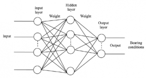
A node layer is a row of the artificial neurons that turn on or off as the input passes through the net (figure 1). The output of each layer is the subsequent layer’s input. The process starts from an initial input layer that receives the data. The number of input and output nodes in an ANN depends on the problem to which the network is being applied. Conversely, there are no fixed rules as to how many nodes the hidden layer should have. If it has few nodes, the network might have difficulty generalizing to problems it has never encountered before; if there are too many nodes, the network may take a long time to learn anything of value [4].
An efficient way to solve complex problems is to decompose the complex system into simpler elements to be able to understand it. On the other side, simple elements can be gathered to produce a complex system. The network structure is one approach to achieve this. Even though there are a number of different types of networks, they can be generalized as having the following components: a set of nodes and connections between them. These can be seen as the computational units, receiving inputs and processing them to obtain an output. The complexity of the processing can vary. It can be simple, like summing the inputs, or complex, in which a node might contain another network, for example. The interactions of the nodes through the connections between them lead to a global behavior of the network. This behavior cannot be observed in the single elements that form the network. This is called an emergent behavior, in which the abilities of the network as a whole supersede the ones of its constitutive elements [6].
ANNs have also some restrictions. Some of its limitations are that there are no structured methodologies available in ANNs, they are not a daily general-purpose problem solver, there is no single standardized paradigm for ANN development, the output quality may be unpredictable, and many ANN systems do not describe how they solve problems [9].
Artificial neural networks and biology
As mentioned previously, the concept of an ANN is inspired and introduced from the subject of biology. Biological neural networks play a vital role processing information in the human body and in other animals. They are formed by trillions of nerve cells (neurons) that exchange brief electrical pulses called action potentials. This web of interconnected neurons is the best example of parallel processing. ANNs, therefore, are computer algorithms that try to mimic these biological structures [2] [9].
The artificial neurons of the ANNs also accept inputs from the other elements or other artificial neurons. After the inputs are weighted and summed, the outcome is transformed by a transfer function into the output. According to Yadav et al. (2013), this transfer function can be a sigmoid, hyperbolic tangent functions, or a step [9].
ANNs are configured for a specific application, like pattern recognition or data classification, through a learning process. The learning in biological systems involves adjustments to the synaptic connections that exist between the neurons. There is an equivalent to this in ANNs, as referred above regarding the weights between the artificial neurons (nodes) [2].
Applications
After the development of the first neural model by McCulloch and Pitts, in 1943, several different models considered ANNs have been developed, that might differ between them in the functions, the accepted values, topology, or learning algorithms for example (6; 8). Traditionally, they have been used to model the human brain and to bring closer the objective of creating an artificial intelligence. Presently, it is common to view ANNs as nonlinear statistical models, or parallel distributed computational systems consisting of many interacting simple elements, or even not having the goal of perfectly modelling the human brain but “to think of feedforward networks as function approximation machines that are designed to achieve statistical generalization, occasionally drawing some insights from what we know about the brain, rather than as models of brain function [1].” In general, NN research has therefore been motivated by the desire to obtain a better understanding of the human brain, and the development of computers that can deal with abstract and poorly defined problems. Conventional computers have difficulty understanding speech and recognizing people’s faces – things that humans do very well [2] [8].
ANNs are an important data mining tool that is used for classification and clustering. They usually learn by example, and when provided with enough examples, the NN should be able to perform classifications, and discover new trends or patterns in the data [4] [8]. They can “help to group unlabeled data according to similarities among the example inputs, and they classify data when they have a labeled dataset to train on [4].” Functionally, ANNs process information, and so they are used in fields related with it, such as modelling real neural networks, and to study behavior and control in animals and machines. They are also used for engineering purposes, such as pattern recognition, forecasting, and data compression, or even for character recognition [2] [6]. The interest in ANNs has increased and are being successfully applied across a range of different domains, in areas as finance (e.g. stock market prediction), medicine, engineering, geology and physics [8].
As with every technology, it is expected that ANNs improve in the future, leading to robots that can see, feel, and predict the world around them, improved stock predictions, self-driving cars, the composition of music , the analysis of handwritten documents that are then automatically transformed into formatted word processing documents, and self-diagnosis of medical problems using NNs [2].
Brief historical context
In 1943, McCullock and Pitts proved that a neuron can have two states. And that those are could be dependent on some threshold value. They presented the first artificial neuron model, and since that time new and more sophisticated models have been presented [8]. According to Kriesel (2007), “Pitts introduced models of neurological networks, recreated threshold switches based on neurons and showed that even simple networks of this kind are able to calculate nearly any logic or arithmetic function [5].”
Kriesel (2007) furthermore divides the historical context of the development of ANNs in four parts: a beginning (1943-1950), a golden age (1951-1969), a period of long silence (1972-1983), and a renaissance (1985-Present).
A detailed account of the history of NNs can be found in the given reference. What follows is just a brief mentioning of some relevant dates adapted from Kriesel (2007) [5].
1949 - Donald O. Hebb formulated the classical Hebbian rule. This represents in its more generalized form the basis of nearly all neural learning procedures.
1957-1958 – Frank Rosenblatt, Charles Wightman and colleagues developed the first successful neurocomputer, called the “Mark I perceptron”.
1960 – Bernard Widrow and Marcian Hoff introduced the ADALINE (ADAptive Linear Neuron), which was a fast and precise adaptive learning system being the first widely commercially used neural network.
1974 – Paul Werbos developed a learning procedure called “backpropagation of error”
1986 – The “backpropagation of error” learning procedure as a generalization of the delta rule was separately developed and published by the Parallel Distributed Processing Group.
Characteristics of ANNs
Artificial neuron networks have a different approach to problem solving than conventional computers. Regular computers follow a set of instructions in order to solve a problem while neural networks process information in a way more similar to that of a human brain. The network is composed of a large number of interconnected units that work in parallel to solve a specific problem. They are not programmed to perform a specific task, but after a specific example has been chosen for the learning stage of the ANN, they improve their own rules, and the more decisions they make, the better decisions may become. [2] [5] [9].
The learning capability of ANNs is one of its most prominent features, being adaptive. From this learning procedure results the capability of NNs to generalize and associate data. After successful training, an ANN can find reasonable solutions for a similar problem of the same class that they were not trained for. It, therefore, has a high degree of fault tolerance against noisy input data, which means NNs can handle errors better than traditional computer programs. On the other side, the fact that NNs have this distributed fault tolerance brings the disadvantage that, at first sight, one cannot realize what an NN knows and performs, or where the fault is. Summarizing, the main characteristics of ANNs are the adaptive learning capability, self-organization, generalization, fault tolerance, distributed memory, and parallel processing [2] [5].
Conventional algorithmic computers and artificial neural networks are not in competition. Instead, they complement each other. Some tasks are better suited to an algorithmic approach, like arithmetic operation, and others to ANNs. Other tasks may require systems that use a combination of the two approaches, in which, normally, a conventional computer is used to supervise a neural network so that the performance is at maximum efficiency [2].
Structure
Neural networks consist of an input, output and one or more hidden layers. The nodes from the input layer are connected to the ones from the hidden layer and, in the same way, every node of the hidden layer is connected to a node in the output layer. Usually, there are weights associated with each connection. The input layer represents the raw information that is introduced into the network, and its nodes are passive, meaning that this layer of the overall NN does not modify the data. They receive a single value on their input and duplicate it to their multiple outputs. In contrast with the input layer, the hidden and output layers are active (2; 8). The signals received by the input layer are sent to the hidden layer, which then modifies the input values using weight values. The result is sent to the output layer. This will also be modified by the weights of the connections between the hidden and output layer. Finally, the output layer process the information received from the previous layer and produces an output that is then processed by an activation function [8].
Throughout the development of ANNs, different neural network structures have been experimented. Some try to replicate the biological systems and others are based on a more mathematical analysis of the problem at hand. The most commonly used structure can be seen in Figure 1, and it consists of the three layers already mentioned. Each layer can contain one or more nodes, and the lines connecting them represent the flow of information. The quality and type of the data, the specific problem the ANN is trying to solve, and some other parameters will influence on the number of nodes chosen for each layer. It has been suggested that selecting the number of nodes for the hidden layer could be a challenging task. Too many nodes in this layer will increase the number of possible computations that the algorithm has to deal with, and few nodes can reduce the learning ability of the algorithm. Therefore, there is the need to achieve a balance. One way to help reach this is to monitor the progress of the ANN during its training stage. If the results are not improving, possibly there will be the need for modification in its structure [8].
Controlling an ANN involves setting and adjusting the weights between nodes. The initial weights are normally randomly set, and then adjusted during the NN training. Some researchers suggest that the weights should not be changed one at a time. Instead, it is recommended to alter the weights simultaneously. Since some ANNs have a high number of nodes, changing them one or two at a time would prevent the adjustment of the NN to achieve the desired results, in a timely manner. The weights update during the NN training, after iterations. This means that, if the results of the NN after the weights have been updated are better than the previous set of weights, than the new values are kept and the iteration goes on. The aim when setting weights should be in finding the right combination of weights that will help minimize the error [8].
The overall network structure of ANNs should be simple and easy. According to Yadav et al. (2013), “There are mainly two types of arrangements recurrent and non-recurrent structure. The Recurrent Structure is also known as Auto associative or Feedback Network and the Non Recurrent Structure is also known as Associative or feed forward Network. In feed forward Network, the signal travel in one direction only but in Feedback Network, the signal travels in both directions by introducing loops in the net [9].”
Feedforward network
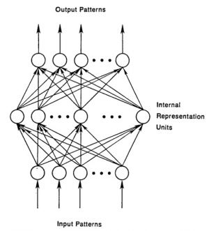
Both feedforward (figure 2) and recurrent networks are named after the way they channel information through a series of mathematical operations that are performed at the nodes of the network. In feedforward networks, the information goes straight through (in a one way), never touching a given node twice, while in the other it cycles it through a loop [7] [10].
The input nodes in feedforward networks do not perform computation and are used instead to distribute inputs into the other layers of the network. In this case, the nodes are grouped in the same layout as described previously: an input layer, one or more hidden processing layers that are invisible from the outside, and an output layer, with each neuron in a layer only having direct connections to the neurons of the next [5] [7].
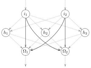
In some feedforward networks, shortcut connections are permitted (figure 3). These connections can skip one or more levels, meaning that they may not only be directed towards the next layer but also towards any other subsequent layer [5].
Recurrent network
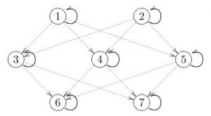
The process of a neuron influencing itself by any means or by any connection is called recurrence. In recurrent networks (figure 4), the input or output neurons may not be explicitly defined. Some networks of this type allow for neurons to be connected to themselves, in a process called direct recurrence (or self-recurrence). When connections towards the input layer from the other layers of the network are allowed, it’s named indirect recurrences. A neuron can use this to influence itself by influencing the neurons of the next layer and these, in turn, will influence it. Lateral recurrences occur when there are connections between neurons within one layer. In this mode, each neuron often will inhibit the other neurons of the layer and strengthen itself, resulting that only the strongest neuron becomes active. Finally, in a recurrent network, there could be a completely linked network. This permits connections between all neurons, except for direct recurrences. Also, the connection has to be symmetric. The neurons are always allowed to be connected to every other neuron, and as a result, every neuron can become an input neuron [5].
The backpropagation algorithm
The backpropagation algorithm is used in layered feedforward ANNs, and it is one of the most popular algorithms. The artificial neurons, organized in layers, send their signals “forward” and the errors are propagated backwards. This algorithm uses supervised learning, in which examples of the inputs and outputs that are intended for the network compute are provided. The error, which is the difference between actual and expected results, is then calculated. The goal of the backpropagation algorithm is to reduce the error, until the ANN learns the training data. The training begins with random weights, and the objective is to adjust them to achieve a minimal error level. Resuming, the backpropagation algorithm can be broken down to four main steps: 1) feedforward computation; 2) back propagation to the output layer; 3) back propagation to the hidden layer, and 4) weight updates [6] [8].
Explain Like I'm 5 (ELI5)
Neural networks are computer programs designed to mimic the human brain's workings. Just as our brain contains millions of tiny neurons working together in synapses to facilitate thoughts and decision-making, a neural network contains many small components called artificial neurons working together in order to solve problems.
When we learn something new, like how to ride a bike, our brain changes the connections between neurons in order to retain what was learned. In a similar fashion, an artificial neural network can alter its artificial neurons' connections in order to learn from data and make better decisions.
For instance, if we want the neural network to recognize photos of cats, then we must show it an extensive library of images of cats and explain what makes a cat a cat. After viewing enough examples, even if it has never seen that particular breed before, the neural network should be able to accurately recognize a picture of a cat as one.
Neural networks are like superhuman computer brains that learn and make decisions independently!
References
- ↑ 1.0 1.1 Zaytsev, O. (2016). A Concise Introduction to Machine Learning with Artificial Neural Networks. Retrieved from http://www.academia.edu/25708860/A_Concise_Introduction_to_Machine_Learning_with_Artificial_Neural_Networks
- ↑ 2.0 2.1 2.2 2.3 2.4 2.5 2.6 2.7 2.8 Nahar, K. (2012). Artificial Neural Network. COMPUSOFT, 1(2): 25-27
- ↑ A basic introduction to neural networks. Retrieved from http://pages.cs.wisc.edu/~bolo/shipyard/neural/local.html
- ↑ 4.0 4.1 4.2 4.3 4.4 4.5 Deeplearning4j. Introduction to deep neural networks. Retrieved from https://deeplearning4j.org/neuralnet-overview.html#introduction-to-deep-neural-networks
- ↑ 5.0 5.1 5.2 5.3 5.4 5.5 5.6 5.7 Kriesel, D. (2007). A Brief Introduction to Neural Networks. Retrieved from http://www.dkriesel.com
- ↑ 6.0 6.1 6.2 6.3 6.4 6.5 Gershenson, C. (2003). Artificial neural networks for beginners. arXiv:cs/0308031v1 [cs.NE]
- ↑ 7.0 7.1 7.2 Dawson, C. W. and Wilby, R. (1998). An artificial neural network approach to rainfall-runoff modelling. Hydrological Sciences Journal, 43(1): 47-66
- ↑ 8.0 8.1 8.2 8.3 8.4 8.5 8.6 8.7 8.8 Cilimkovic, M. Neural networks and back propagation algorithm. Institute of Technology Blanchardstown, Ireland
- ↑ 9.0 9.1 9.2 9.3 9.4 Yadav, J. S., Yadav, M. and Jain, A. (2013). Artificial neural network. International Journal of Scientific Research and Education, 1(6): 108-118
- ↑ Deeplearning4j. A beginner’s guide to recurrent networks and LSTMs. Retrieved from http://deeplearning4j.org/lstm#a-beginners-guide-to-recurrent-networks-and-lstms
