

Degrees of Freedom
Degrees of freedom (DoF) count independent ways in which a system, estimate, or model can vary, but the phrase does not denote one universal quantity. In mechanics and robotics, it usually means the dimension of a configuration space: the minimum number of independent coordinates needed to specify a configuration locally. In statistics, it may mean the dimension of a residual subspace, a parameter of a sampling distribution, or an effective measure attached to a fitting procedure. In control theory, it can refer either to physical motion and actuation or, in phrases such as "two-degree-of-freedom controller," to independently shaped signal paths. These uses share an idea of independent variation, but their numbers are not interchangeable.
The object being counted matters as much as the number. A six-axis robot may have six joint coordinates, fewer than six instantaneous Cartesian directions at a singular configuration, and still fewer independently commanded inputs if some joints are passive. A regression may fit many coefficients while having lower effective degrees of freedom because of shrinkage. Conversely, an adaptive model-selection procedure can have effective degrees of freedom greater than the number of coefficients retained in one fitted model. A useful statement therefore names the space, constraints, operating point, and counting rule.
Core idea
A coordinate list is not automatically a list of degrees of freedom. Coordinates can be redundant, and constraints can make some coordinate changes dependent on others. Suppose a configuration is described by q in an n-dimensional coordinate space and must satisfy smooth equality constraints
At a regular configuration, the local number of configuration degrees of freedom is
If there are k locally independent constraints, then the rank of Dg(q) is k, giving n-k degrees of freedom. Counting equations instead of their independent rank can give the wrong answer when constraints are redundant. The rank can also change at exceptional configurations, so a mechanism can behave differently at singular or specially aligned positions.[1][3][7]
This local dimension is distinct from several related counts:
| Quantity | What it counts | Why it can differ |
|---|---|---|
| Configuration DoF | Independent coordinates needed to specify configuration | Depends on geometric constraints and the configuration manifold |
| Joint or generalized-coordinate count | Variables selected to describe a mechanism | May contain dependent or redundant coordinates |
| Instantaneous task mobility | Independent task-space velocities available at one configuration | Depends on the rank of a Jacobian at that configuration |
| Actuation count | Independently commandable inputs | Passive, coupled, or failed actuators can make it smaller than configuration DoF |
| Residual statistical DoF | Independent directions left after fitting constraints | Depends on the rank of the fitted model |
| Distributional DoF | Shape parameter of a reference distribution | Comes from a derivation, not simply from counting columns |
| Effective model DoF | Sensitivity or optimism of a fitting procedure | Can be fractional and can depend on the data-generating mean and tuning procedure |
The word "independent" is therefore mathematical, not merely descriptive. Two motions that look different may be coupled by a constraint. Two estimated parameters may also represent only one estimable direction if their columns in a design matrix are linearly dependent.
Mechanical degrees of freedom
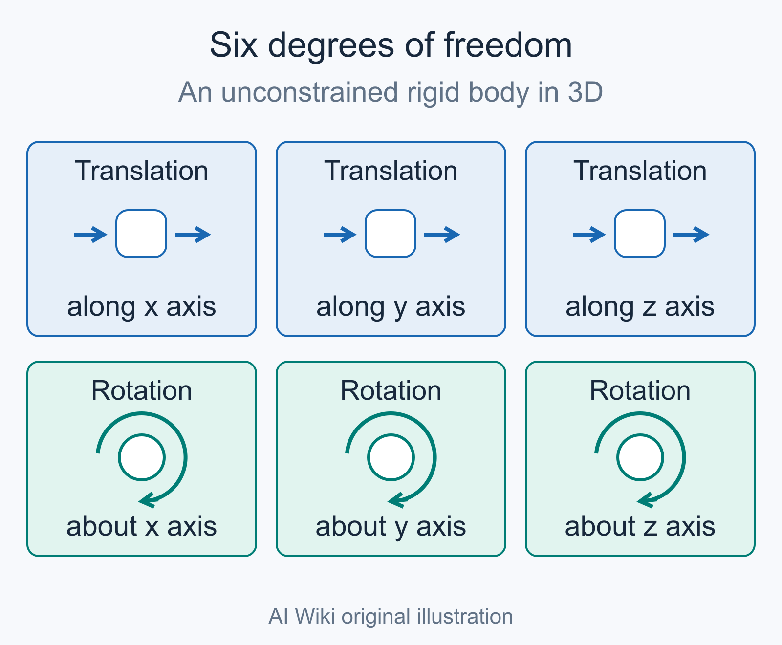
An unconstrained rigid body in three-dimensional space has three translational and three rotational degrees of freedom. The small icons identify motion categories; they are not axis-specific perspective drawings. Constraints can reduce the number of independent motions.[22] Illustration: AI Wiki original diagram. CC0 1.0.
Rigid bodies
A free rigid body in three-dimensional space has six configuration degrees of freedom: three for translation and three for orientation. A planar rigid body has three: two translations and one rotation. These statements concern the dimension of the configuration space, not a globally valid choice of six or three unconstrained real numbers. Orientation coordinates can have singularities or redundancy even though the rotation space itself has dimension three.[1]
A joint removes relative motions between two bodies while leaving specified motions possible. An ideal revolute joint contributes one relative rotational DoF, and an ideal prismatic joint contributes one relative translational DoF. A spherical joint contributes three rotational DoF. These are ideal kinematic descriptions. Compliance, backlash, deformation, contact, and manufacturing tolerances can introduce motions that are important physically without being intended configuration coordinates.[2]
For a mechanism with N links including the fixed link, J joints, and joint i permitting f_i relative freedoms, the generic Gruebler-Kutzbach count is
where m=3 for planar mechanisms and m=6 for spatial mechanisms. This is a constraint count, not an infallible test. It assumes the constraints contributed by the joints have the expected independent rank. Special geometry can make constraints dependent and produce an overconstrained mechanism whose actual mobility is greater than the generic formula predicts. Direct constraint analysis, screw-theoretic analysis, or a Jacobian-rank calculation is then required.[2][7]
The formula also does not say whether a nominal motion is usable over a finite range. Joint limits, collisions, contact loss, or disconnected components of configuration space can restrict reachable configurations without changing the local dimension at an ordinary interior point.
Holonomic and nonholonomic constraints
A holonomic constraint can be written as an equality involving configuration variables, such as g(q)=0. Under regularity and independence conditions, it reduces the dimension of the configuration space. A nonholonomic constraint restricts allowable velocities but cannot, in the relevant neighborhood, be integrated into an equivalent configuration-only equality. The rolling-without-slipping constraint of a wheeled vehicle is the standard example: the vehicle cannot move instantaneously sideways, yet sequences of admissible forward and turning motions can change its lateral position.[3][8]
This distinction prevents a common counting error. The number of instantaneous velocity directions is not always the same as the dimension of the set of configurations reachable by a sequence of motions. A differential-drive mobile robot has a three-dimensional planar pose even though its no-slip model permits only two independent velocity inputs at an instant. Reachability then depends on the structure of the velocity constraints, not only on subtracting their number from the configuration dimension.[3][8]
Contact can change the count during operation. A free body has one configuration space, while the same body resting against a surface or grasped at several contacts has additional constraints. If a robot establishes or breaks contacts, as in walking or manipulation, its model can pass among contact modes with different admissible velocities and possibly different local configuration dimensions. Any reported DoF count should say which contacts are assumed active.
Degrees of freedom in robotics
Configuration, task, and workspace
Robot descriptions often use DoF as shorthand for the number of joints, but that is safe only when the joint coordinates are independent and form a minimal description. A serial manipulator with n independent one-DoF joints has an n-dimensional configuration space away from identifications and limits. A closed-chain mechanism can have many joint variables but fewer independent configuration coordinates because loop-closure constraints couple them.[2]
Task space describes the variables relevant to a task, not every robot coordinate. The pose of a rigid end effector in space is a six-dimensional task variable, but reaching a point without prescribing orientation uses a three-dimensional position task. A camera pointing task, a welding path, and a mobile-base pose each define different task variables. Workspace is the set of task-space values the robot can actually attain, given its geometry and constraints. Configuration space and task space are therefore neither synonyms nor required to have the same dimension.[4]
This distinction is essential when comparing robots. Saying that one robot has more degrees of freedom does not by itself establish a larger workspace, greater payload, better precision, or higher task success. Extra configuration coordinates may help avoid obstacles, satisfy joint limits, or maintain a preferred posture, but they also add sensing, calibration, planning, and control requirements. Capability depends on geometry, actuation, limits, sensing, control, and the task definition, not on a DoF total alone.
Jacobian rank, singularity, and redundancy
For a differentiable task map x=f(q), the Jacobian relates joint velocity to task velocity:
At a fixed configuration, the attainable instantaneous task-velocity space is the range of J(q), so its dimension is the rank of J(q). If the Jacobian loses rank, the robot is at a kinematic singularity for that task: at least one task-space direction that is available nearby may be unavailable instantaneously, and forces or joint rates associated with some commands can become ill-conditioned.[5]
When a robot has n independent configuration velocities and the rank of J(q) is r, the null space has dimension
Null-space motion changes the robot configuration without changing the chosen task variable to first order. This is the precise local sense in which a robot is redundant for a task. Redundancy is task-dependent. A seven-joint arm can be redundant for a six-dimensional end-effector pose task at a regular configuration, but it need not be redundant after additional objectives or constraints are imposed. At a singularity, the task rank can fall and the nullity can rise, yet the loss of task directions is a limitation rather than a capability gain.[5][6]
The singular values of J, obtainable through singular value decomposition, describe local directional scaling. Small singular values identify task directions requiring large joint velocities for a given task velocity. Manipulability measures summarize aspects of this local geometry, but their value depends on coordinate units, scaling, configuration, and the particular Jacobian used. They are not universal robot rankings.[6]
Actuation and underactuation
Configuration DoF and actuator count answer different questions. A fully actuated mechanical system has enough independent control authority, under the adopted model, to command generalized forces across its configuration directions. A common sign of underactuation is fewer independent inputs than configuration coordinates, but input rank, contact state, actuator limits, and dynamics also matter. A floating-base legged robot, for example, gains six configuration coordinates for the unanchored base without gaining six direct base actuators. Ground contact can provide constraint forces, but those forces are conditional on contact and friction.[8]
An actuator count can also overstate effective control authority if transmissions couple joints or the input map loses rank. Conversely, an underactuated system may still be controllable over time by exploiting dynamics. Underactuated does not mean uncontrolled, and fully actuated does not guarantee that every state can be reached safely under limits.
These distinctions affect motion planning. A path in configuration space specifies a geometric sequence of configurations. A dynamically feasible trajectory also assigns time and satisfies velocity, acceleration, force, contact, and input constraints. Adding configuration DoF generally enlarges the decision space, but it does not imply one fixed computational scaling law. Difficulty depends on obstacle geometry, constraints, representation, algorithm, and the structure a planner can exploit.
Statistical degrees of freedom
In statistics, degrees of freedom usually arise from the number of independent random directions remaining after constraints, or as a parameter in a derived sampling distribution. The familiar rule "number of observations minus number of estimated parameters" is correct for important full-rank linear cases, but it is not a universal definition.
Sample variance and the t distribution
For independent normally distributed observations Y_1,...,Y_n with common mean mu and variance sigma^2, the deviations from the sample mean satisfy
Only n-1 of those deviations can vary independently. Under the normal model,
Estimating the mean has removed one residual direction. Student's one-sample statistic uses the same variance estimate and, under these assumptions, has a t distribution with n-1 degrees of freedom.[9][10]
The assumptions are part of the statement. Correlation among observations, unequal variance, weighting, clustering, missing-data procedures, or estimating additional quantities can change the relevant reference distribution and its degrees of freedom. Merely counting records does not resolve those issues.
Linear models and rank
Consider the linear regression model
with n observations and a design matrix X of rank r. Ordinary least squares projects y onto the r-dimensional column space of X. The fitted values have model degrees of freedom r, while the residual vector lies in an orthogonal subspace of dimension n-r. The residual degrees of freedom are therefore n-r, not necessarily n-p, where p is the number of columns. The two coincide only when all p columns are linearly independent.[15]
This rank formulation handles redundant parameterizations. If two columns are identical, two named coefficients do not create two independent fitted directions. Some coefficient vectors may be nonunique even though the fitted vector is unique. Estimability and residual variation are properties of the relevant subspaces.
For nested least-squares models, an F statistic compares reductions in residual sum of squares relative to the dimensions added and left over. In one-way analysis of variance with k groups and N total observations, the standard fixed-effects decomposition assigns k-1 degrees of freedom to between-group variation, N-k to within-group error, and N-1 in total. These formulas assume the usual model structure and do not transfer unchanged to repeated-measures, mixed, or unbalanced designs with other estimators.[11]
Distributional and approximate degrees of freedom
The chi-square, t, and F families use degrees of freedom as distribution parameters. Those parameters often have geometric derivations from independent normal components or residual subspaces, but a reported value should come from the test or estimator actually used.
Degrees of freedom need not be an integer. In the unequal-variance two-sample t procedure, the Welch-Satterthwaite approximation replaces the exact, generally non-t reference distribution of the standardized mean difference with a t distribution whose degrees of freedom are
The resulting nu is usually fractional. It is an approximation chosen to match moments of an estimated variance, not a literal count of observations that remain free.[12][13]
Contingency-table tests offer another constrained count. In an R by C table under a standard independence model with fixed sample size, estimating row and column margins leaves (R-1)(C-1) degrees of freedom for departures from independence. Sparse expected counts and data-dependent category choices affect the validity of the chi-square approximation even when the algebraic count is unchanged.[14]
Effective degrees of freedom in statistical learning
Machine learning and modern regression methods frequently use shrinkage, smoothing, or adaptive variable selection. The number of coefficients stored by the algorithm may then be a poor description of how strongly the fitted values respond to the observed responses.
For observations y=mu+epsilon with independent errors of common variance sigma^2, one widely used definition is
This definition measures the optimism of in-sample squared error relative to prediction error under its stated setup. It depends on the fitting procedure and can also depend on the unknown mean mu. It is not automatically a count of trainable parameters.[15][16]
If the fitted values are produced by a fixed linear smoother, mu_hat=Sy, then
For ordinary least squares, S is an idempotent projection and its trace equals its rank. For ridge regression with a fixed penalty lambda,
Shrinkage makes the trace generally fractional and smaller than the rank of an unpenalized full fit for positive lambda, subject to the treatment of an intercept and any unpenalized terms. This connects effective DoF to the bias-variance tradeoff, but it does not turn the trace into a universal measure of model complexity.[16][17]
Adaptive methods require more care. For the lasso under a Gaussian linear-model setup and a fixed tuning parameter, the degrees of freedom of the fitted response can be expressed as the expected rank of the selected predictor columns. Under suitable full-rank conditions, this reduces to the expected active-set size. The active-set size from one realized dataset is therefore an estimator or realization-dependent quantity, not a universal identity for every design, noise model, or tuning process.[18][19]
Variable search itself can consume degrees of freedom. Best-subset selection and forward stepwise procedures choose a model after seeing the same responses used for fitting. Their effective degrees of freedom can exceed the number of coefficients in the selected model, and for some nonconvex projection procedures can even exceed the ambient response dimension. Effective DoF is consequently useful for prediction-error calculations, but it need not be monotone in an intuitive model-size parameter.[15][20]
This limitation is especially important when a tuning parameter is selected from the data. Formulas derived for a fixed penalty or fixed smoothing parameter do not automatically include the additional adaptivity of cross-validation, stopping rules, architecture search, or feature screening. A report should say whether it treats the tuning choice as fixed or accounts for selection.
The phrase "effective degrees of freedom" is also used in other senses, including corrections for autocorrelated samples and approximations in mixed models. Those definitions solve different inferential problems. A numerical effective sample size, a Satterthwaite denominator DoF, and the covariance-based DoF of a fitted predictor should not be substituted for one another merely because all are abbreviated "EDF."
Control terminology
Mechanical DoF, actuation, and controller-architecture DoF are separate concepts. A plant can have several configuration coordinates but only a smaller number of independent inputs. Engineers may analyze the rank and structure of the input map, controllability over time, and input constraints rather than equating input count with mechanical mobility.[8]
In controller design, a two-degree-of-freedom structure commonly provides separately adjustable paths for response to a reference command and response to disturbances or measurement feedback. For example, a feedback compensator can be paired with a reference prefilter or feedforward element. The "two" labels independently shapeable closed-loop transfer relationships; it does not mean the controlled mechanism has two joints or two spatial motion coordinates.[21]
The same warning applies to phrases such as control allocation or redundant actuation. More actuators than task variables may provide choices for distributing effort, respecting limits, or tolerating a failure, but the usable allocation freedom is determined by the rank of the effectiveness map and active constraints. Counts should be evaluated at the operating condition represented by that map.
Interpretation and reporting
A degrees-of-freedom claim is interpretable when it answers four questions:
- What object varies? Examples include a mechanism configuration, an instantaneous end-effector velocity, a residual vector, a reference distribution, or fitted responses.
- What constraints or estimator apply? State joint closures, contacts, design-matrix rank, distributional assumptions, penalty, tuning rule, or controller structure.
- Is the claim local, global, or approximate? Jacobian rank is local to a configuration; workspace is global; Welch-Satterthwaite DoF is an approximation.
- What counting rule is used? Name dimension, matrix rank, actuator-input rank, distribution parameter, trace of a smoother, or covariance-based effective DoF.
For robots, it is clearer to report configuration DoF, task dimension, Jacobian rank at the relevant pose, independent actuator inputs, and active contacts separately. Product phrases such as "seven-DoF arm" usually describe nominal joint axes, not all of these quantities. For statistical work, reports should identify whether a number is residual, numerator, denominator, distributional, or effective degrees of freedom and should state the model and approximation that produced it.
Degrees of freedom are most useful as a compact summary after the mathematical object has been specified. Used without that context, the same phrase can conceal rather than clarify the distinction among coordinates, reachable motions, control authority, residual information, and estimator adaptivity.
References
- ^1 ^2Lynch, Kevin M., and Frank C. Park. "Degrees of Freedom of a Rigid Body." *Modern Robotics* companion resource, Northwestern University. modernrobotics.northwestern.edu/...of-a-rigid-body
- ^1 ^2 ^3Lynch, Kevin M., and Frank C. Park. "Degrees of Freedom of a Robot." *Modern Robotics* companion resource, Northwestern University. modernrobotics.northwestern.edu/...edom-of-a-robot
- ^1 ^2 ^3Lynch, Kevin M., and Frank C. Park. "Configuration and Velocity Constraints." *Modern Robotics* companion resource, Northwestern University. modernrobotics.northwestern.edu/...ity-constraints
- ^Lynch, Kevin M., and Frank C. Park. "Task Space and Workspace." *Modern Robotics* companion resource, Northwestern University. modernrobotics.northwestern.edu/...e-and-workspace
- ^1 ^2Lynch, Kevin M., and Frank C. Park. "Singularities." *Modern Robotics* companion resource, Northwestern University. modernrobotics.northwestern.edu/...5-3-singularities
- ^1 ^2Lynch, Kevin M., and Frank C. Park. "Manipulability." *Modern Robotics* companion resource, Northwestern University. modernrobotics.northwestern.edu/...-manipulability
- ^1 ^2Dai, Jian S., Zhen Huang, and Harvey Lipkin. "Mobility of Overconstrained Parallel Mechanisms." *Journal of Mechanical Design* 128, no. 1 (2006): 220-229. doi.org/...1.1901708
- ^1 ^2 ^3 ^4Tedrake, Russ. "Underactuated Robotics: Learning, Planning, and Control for Efficient and Agile Machines." MIT course notes, chapter 1. underactuated.mit.edu/intro
- ^Student. "The Probable Error of a Mean." *Biometrika* 6, no. 1 (1908): 1-25. doi.org/...2331554
- ^NIST/SEMATECH. "t Distribution." *e-Handbook of Statistical Methods*. itl.nist.gov/...eda3664
- ^NIST/SEMATECH. "One-Way ANOVA." *e-Handbook of Statistical Methods*. itl.nist.gov/...ppc231
- ^Welch, B. L. "The Generalization of Student's Problem When Several Different Population Variances Are Involved." *Biometrika* 34, nos. 1-2 (1947): 28-35. doi.org/...34.1-2.28
- ^Satterthwaite, Franklin E. "An Approximate Distribution of Estimates of Variance Components." *Biometrics Bulletin* 2, no. 6 (1946): 110-114. doi.org/...3002019
- ^Fisher, R. A. "On the Interpretation of Chi Square from Contingency Tables, and the Calculation of P." *Journal of the Royal Statistical Society* 85, no. 1 (1922): 87-94. doi.org/...2340521
- ^1 ^2 ^3Janson, Lucas, William Fithian, and Trevor J. Hastie. "Effective Degrees of Freedom: A Flawed Metaphor." *Biometrika* 102, no. 2 (2015): 479-485. doi.org/...asv019
- ^1 ^2Efron, Bradley. "How Biased Is the Apparent Error Rate of a Prediction Rule?" *Journal of the American Statistical Association* 81, no. 394 (1986): 461-470. doi.org/...01621459.1986.10478291
- ^Golub, Gene H., Michael Heath, and Grace Wahba. "Generalized Cross-Validation as a Method for Choosing a Good Ridge Parameter." *Technometrics* 21, no. 2 (1979): 215-223. doi.org/...00401706.1979.10489751
- ^Zou, Hui, Trevor Hastie, and Robert Tibshirani. "On the Degrees of Freedom of the Lasso." *The Annals of Statistics* 35, no. 5 (2007): 2173-2192. doi.org/...009053607000000127
- ^Tibshirani, Ryan J., and Jonathan Taylor. "Degrees of Freedom in Lasso Problems." *The Annals of Statistics* 40, no. 2 (2012): 1198-1232. doi.org/...12-AOS1003
- ^Tibshirani, Ryan J. "Degrees of Freedom and Model Search." *Statistica Sinica* 25, no. 3 (2015): 1265-1296. doi.org/...ss.2014.147
- ^Taguchi, Hidefumi, and Mituhiko Araki. "Two-Degree-of-Freedom PID Controllers: Their Functions and Optimal Tuning." *IFAC Proceedings Volumes* 33, no. 4 (2000): 91-96. doi.org/...S1474-6670(17)38226-5
- ^AI Wiki. "Six degrees of freedom". CC0 1.0. Original geometric illustration; not a reproduction of a source figure. Technical basis: Lynch and Park, Degrees of Freedom of a Rigid Body.
Improve this article
Add missing citations, update stale details, or suggest a clearer explanation. Every suggestion is reviewed for sourcing before it goes live.
5 revisions · v6 · 3,694 words · full history
Fact-checks are independent of edits: a reviewer re-verifies the article against its sources and stamps the date. How we verify
Research and drafting on this wiki are AI-assisted, under named human editorial standards. How AI is used here
Reviewer note: Independently verified against 21 primary, peer-reviewed, official, and authoritative records covering mechanics, robotics, statistics, statistical learning, control terminology, equations, assumptions, and bibliographic metadata; technical, mathematical, numerical, and currentness claims checked through 2026-07-28.
Cite this page: AI Wiki. "Degrees of Freedom." aiwiki.ai, updated 28 Jul 2026, fact-checked 28 Jul 2026. CC BY 4.0. https://aiwiki.ai/wiki/degrees_of_freedom