

Kernel trick
The kernel trick is a technique in machine learning for turning an algorithm that is linear in its inputs into a nonlinear one: every inner product between two data points is replaced by a kernel function $k(x, x')$ that equals the inner product of the points after a mapping $\Phi$ into a (usually much higher-dimensional) feature space, so the algorithm behaves as if it were run in that space without ever computing $\Phi(x)$ [1][2]. The functions that can play this role are exactly the positive definite kernels, and some of them, such as the Gaussian kernel, correspond to inner products in infinite-dimensional spaces while still being cheap to evaluate [1][4]. The idea underlies support vector machines with nonlinear kernels, kernel principal component analysis, kernel ridge regression and Gaussian process regression, and it reappears in modern work on the neural tangent kernel and on linear attention for transformers [1][11][15][16].
The name is informal. Hofmann, Schölkopf and Smola's 2008 review in The Annals of Statistics describes the substitution of $k(x, x')$ for $\langle \Phi(x), \Phi(x') \rangle$ as what "the machine learning community" calls the kernel trick, and Rasmussen and Williams' textbook on Gaussian processes says the technique "is sometimes called the kernel trick" [1][2].
How the kernel trick works
Feature maps and kernels
Many learning methods, from linear regression to the perceptron, fit a function that is linear in the input vector $x$. A standard way to make them fit nonlinear patterns is to apply a feature map $\Phi$ that sends each input to a new vector of features (for example, all products of pairs of coordinates) and then run the linear method on $\Phi(x)$ instead of $x$ [4]. The model is still linear in the features, but nonlinear in the original inputs [1][4].
The drawback is cost. The Stanford CS229 lecture notes by Tengyu Ma and Andrew Ng give the example of a feature map containing all monomials of degree up to 3 in a $d$-dimensional input: the feature vector has on the order of $d^3$ entries, so for $d = 1000$ each gradient update must compute and store a vector of about $10^9$ numbers [4].
A kernel is a function $k : \mathcal{X} \times \mathcal{X} \to \mathbb{R}$ that satisfies
for some feature map $\Phi$ into an inner product space $\mathcal{H}$, called the feature space [1]. If an algorithm touches the data only through inner products $\langle x, x' \rangle$, each of those inner products can be replaced with $k(x, x')$, and the algorithm then runs implicitly in $\mathcal{H}$ [2][4]. Rasmussen and Williams note that this is particularly valuable when the kernel is more convenient to compute than the feature vectors, and that it often leads to treating the kernel as the object of primary interest and the feature space as having secondary practical importance [2].
A worked example: the polynomial kernel
For $x, z \in \mathbb{R}^d$, the kernel $k(x, z) = (x^\top z)^2$ expands to
which is the inner product of two feature vectors whose entries are all $d^2$ pairwise products $x_i x_j$ [4]. Computing those feature vectors explicitly takes $O(d^2)$ time, but computing $(x^\top z)^2$ takes only $O(d)$, because it needs just one ordinary inner product and a square [4]. Adding a constant, $k(x, z) = (x^\top z + c)^2$, adds the first-order terms $\sqrt{2c},x_i$ and a constant feature, with $c$ controlling the relative weight of first-order and second-order terms [4].
The same pattern holds at any degree. Hofmann and colleagues show that the homogeneous kernel $\langle x, x' \rangle^p$ is the inner product between vectors listing all ordered products of $p$ input coordinates, and that the inhomogeneous kernel $(\langle x, x' \rangle + c)^p$ with $c \geq 0$ covers all monomials up to degree $p$ [1]. The CS229 notes put the dimension of that space at $\binom{d+k}{k}$ for degree $k$, of order $d^k$, while the kernel itself still costs $O(d)$ to evaluate [4].
Kernelizing an algorithm
To apply the trick, an algorithm has to be rewritten so that the data appear only inside inner products. The CS229 notes do this for least-mean-squares regression trained by gradient descent. Starting from zero weights, every update adds a linear combination of the mapped training points $\Phi(x^{(i)})$, so the weight vector can always be written as $\theta = \sum_{i=1}^{n} \beta_i \Phi(x^{(i)})$ [4]. The update can then be carried out on the coefficients alone,
where $K$ is the $n \times n$ matrix with entries $K_{ij} = k(x^{(i)}, x^{(j)})$, and a prediction is $\theta^\top \Phi(x) = \sum_i \beta_i , k(x^{(i)}, x)$ [4]. The feature vectors never appear. The notes add that the same substitution yields a kernel perceptron and works for any learning algorithm that can be written purely in terms of inner products between inputs [4].
Hofmann and colleagues give a second example: a classifier that assigns a point to the class whose mean is closer in feature space. Expanding the class means $c_+$ and $c_-$ turns the rule into
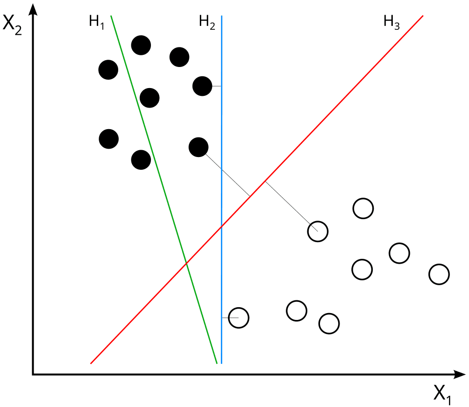
where $n_+$ and $n_-$ count the examples in each class and the offset $b$ is also a sum of kernel values [1]. The decision boundary is a hyperplane in feature space but a nonlinear curve in the input space, and the review describes this classifier as closely related to the support vector machine [1].
Which functions are valid kernels
Gram matrices and positive definiteness
Given a kernel $k$ and inputs $x_1, \dots, x_n$, the $n \times n$ matrix $K_{ij} = k(x_i, x_j)$ is called the Gram matrix or kernel matrix [1]. A function $k$ is a positive definite kernel if, for every finite set of inputs, its Gram matrix is symmetric and satisfies $\sum_{i,j} c_i c_j K_{ij} \geq 0$ for all real coefficients $c_i$ [1]. Terminology varies: Hofmann and colleagues call this condition "positive definite" and reserve "strictly positive definite" for the case where equality holds only when all $c_i$ are zero, while the CS229 notes describe the same requirement as the kernel matrix being symmetric positive semidefinite [1][4].
The central result is that the functions which can be written as $\langle \Phi(x), \Phi(x') \rangle$ are exactly the positive definite kernels [1]. One direction is short: any kernel of that form gives $\sum_{i,j} c_i c_j k(x_i, x_j) = \lVert \sum_i c_i \Phi(x_i) \rVert^2 \geq 0$ [1][4]. The CS229 notes state the converse as a theorem due to Mercer: a function is a valid kernel if and only if every finite kernel matrix it produces is symmetric positive semidefinite [4]. This gives a practical test: a candidate similarity function can be checked for validity without ever writing down its feature map [4]. Positive definite kernels also obey a Cauchy-Schwarz inequality, $k(x_1, x_2)^2 \leq k(x_1, x_1), k(x_2, x_2)$ [1].
Reproducing kernel Hilbert spaces
For the converse direction, Hofmann and colleagues construct the feature space explicitly. Each input $x$ is mapped to the function $k(\cdot, x)$, finite combinations $f = \sum_i \alpha_i k(\cdot, x_i)$ are given the inner product $\langle f, g \rangle = \sum_{i,j} \alpha_i \beta_j k(x_i, x'_j)$, and completing this space yields a Hilbert space of functions [1]. In that space the kernel has the reproducing property
which is why $k$ is called a reproducing kernel and the space a reproducing kernel Hilbert space (RKHS) [1]. The Moore-Aronszajn theorem, from N. Aronszajn's 1950 paper "Theory of reproducing kernels", states that every positive definite kernel has a unique RKHS and vice versa [1][6]. The RKHS view also matters for regularization: the squared norm $\lVert f \rVert_{\mathcal{H}}^2$ is the penalty used by support vector machines, and for translation-invariant kernels it can be read in the Fourier domain, where frequencies at which the kernel's Fourier transform is small are penalized strongly; kernels whose transform decays at high frequencies therefore favor smooth functions [1].
Mercer's theorem
James Mercer's 1909 memoir in the Philosophical Transactions of the Royal Society set out to find conditions under which a symmetric continuous function $k(s, t)$ is "definite" in Hilbert's sense, and ended up studying the wider classes of functions of "positive and negative type" [5]. In the form given by Rasmussen and Williams, Mercer's theorem says that, for a kernel whose integral operator is positive definite on a finite measure space, the kernel can be expanded in the operator's eigenfunctions $\phi_i$ and eigenvalues $\lambda_i > 0$,
with absolutely summable eigenvalues and a series that converges absolutely and uniformly almost everywhere [3]. Rasmussen and Williams describe this as the infinite-dimensional analogue of diagonalizing a Hermitian matrix, and note that the eigenfunctions of a kernel can serve as a set of basis functions, so that Gaussian process regression can be viewed as Bayesian linear regression with a possibly infinite number of them [3].
Early kernel-machine papers characterized valid kernels by Mercer's conditions, and kernels satisfying them are often called Mercer kernels [1][4]. Hofmann and colleagues point out that every such kernel can be written as an inner product but the converse does not hold, so positive definite kernels, rather than Mercer kernels, are the natural class for the kernel trick [1].
Building new kernels
Positive definite kernels are closed under several operations, which lets practitioners assemble kernels from simpler pieces [1]:
- Nonnegative combinations $\alpha_1 k_1 + \alpha_2 k_2$ with $\alpha_1, \alpha_2 \geq 0$, and pointwise limits of kernels, are kernels.
- The pointwise product $k_1 k_2$ is a kernel.
- Tensor products and direct sums of kernels on two domains are kernels on the product domain.
- A function of an inner product, $\psi(\langle x, x' \rangle)$, is a kernel in every Hilbert space if and only if $\psi$ is a power series with nonnegative coefficients.
The last result gives a short proof that the Gaussian kernel is valid: $e^{\langle x, x' \rangle / \sigma^2}$ is a kernel because the exponential series has positive coefficients, and multiplying it by $f(x) f(x')$ with $f(x) = e^{-\lVert x \rVert^2 / 2\sigma^2}$ yields $e^{-\lVert x - x' \rVert^2 / (2\sigma^2)}$ [1]. For kernels that depend only on $x - x'$, Bochner's theorem characterizes validity: a continuous function $h$ on $\mathbb{R}^d$ is positive definite if and only if it is the Fourier transform of a finite nonnegative measure, and the Gaussian kernel corresponds to a normal distribution over frequencies [1]. Rahimi and Recht's random Fourier features, described below, are built on this theorem [13].
Hofmann and colleagues also describe a larger class, conditionally positive definite kernels, whose Gram matrices only need to satisfy the positivity condition for coefficients summing to zero; it is the analogue of the kernel trick for distances rather than similarities, and support vector machines and kernel PCA can be used with such kernels as well [1].
Common kernels
| Kernel | Formula | Notes |
|---|---|---|
| Linear | $x^\top x'$ | Polynomial kernel of degree 1 with no offset; the feature map is the identity [1][10] |
| Polynomial | $(\gamma x^\top x' + c_0)^d$ | Homogeneous when $c_0 = 0$; features are monomials of the inputs [1][10] |
| Gaussian (RBF) | $\exp(-\gamma \lVert x - x' \rVert^2)$ | Infinite-dimensional feature map; strictly positive definite [1][4][10] |
| Laplacian | $\exp(-\gamma \lVert x - x' \rVert_1)$ | RBF variant using Manhattan distance [10] |
| Matérn | Bessel-function form with smoothness $\nu$ | Recommended by Stein over the Gaussian for many physical processes, per Rasmussen and Williams [3] |
| Rational quadratic | $(1 + r^2 / (2\alpha\ell^2))^{-\alpha}$, $r = \lVert x - x' \rVert$ | Stationary covariance function used with Gaussian processes [3] |
| Sigmoid | $\tanh(\gamma x^\top x' + c_0)$ | Also called the hyperbolic tangent or multilayer perceptron kernel, after the neural network activation function; Rasmussen and Williams state it is never positive definite [3][10] |
| Chi-squared | $\exp(-\gamma \sum_i (x_i - x'_i)^2 / (x_i + x'_i))$ | For nonnegative histogram features, common in computer vision [10] |
| String kernels | Weighted counts of shared substrings | Exact-match versions computable in $O(\lvert x \rvert + \lvert x' \rvert)$ with suffix trees [1] |
| Graph diffusion kernel | $\exp(-\lambda L)$ for graph Laplacian $L$ | Similarity between vertices of a graph [1] |
| Fisher kernel | Inner product of Fisher scores of a probabilistic model | Built from a probability density model $p(x \mid \theta)$ [1] |
Rasmussen and Williams call the Gaussian (which they name the squared exponential) "probably the most widely-used kernel within the kernel machines field", and show that it can be derived as the limit of a model with infinitely many Gaussian-shaped basis functions placed densely along the input space [3]. Its bandwidth parameter sets how quickly similarity decays with distance: scikit-learn writes it as $\exp(-\gamma \lVert x - x' \rVert^2)$, which matches the form $\exp(-\lVert x - x' \rVert^2 / 2\sigma^2)$ when $\gamma = 1/(2\sigma^2)$ [1][10].
A notable property of the kernel trick is that the inputs do not need to be vectors at all. Because the algorithm only consults $k(x, x')$, kernels can be defined on strings, trees, graphs, sets and probability distributions [1]. Hofmann and colleagues list applications of string and tree kernels in document categorization, spam filtering, protein function prediction, DNA annotation and parse-tree construction [1].
The representer theorem
The representer theorem explains why kernelized algorithms can work with finite sums even when the feature space is infinite-dimensional. In the form stated by Hofmann and colleagues, for any loss function $c$ evaluated on the training points and any strictly increasing function $\Omega$ of the RKHS norm, every minimizer of the regularized risk
can be written as
[1]. The result traces to George Kimeldorf and Grace Wahba's 1971 work on spline functions [1][7]. Its practical meaning is that the search over a space of functions reduces to a search over $n$ coefficients, one per training example; in support vector machines this is the support vector expansion, and for suitable loss functions many of the $\alpha_i$ are zero [1]. The flip side is that prediction time grows with the number of nonzero terms, which can be large in practice [1].
Algorithms that use the kernel trick
| Method | Linear starting point | Notes |
|---|---|---|
| Kernel support vector machine | Maximum-margin hyperplane (the generalized portrait) | Boser, Guyon and Vapnik, 1992 [1][8] |
| Kernel principal component analysis | Principal component analysis | Schölkopf, Smola and Müller, 1998 [1][9] |
| Kernel ridge regression | Ridge regression | Closed-form fit; dense solution [11] |
| Gaussian process regression | Bayesian linear regression | The kernel serves as the covariance function [2][3] |
| Kernel perceptron | Perceptron | Same substitution applied to perceptron updates [4] |
| Kernel canonical correlation and independence measures | Canonical correlation analysis | Used for independent component analysis by Bach and Jordan [1] |
In kernel PCA, the covariance matrix of the mapped data cannot be diagonalized directly in feature space, but its eigenvectors lie in the span of the mapped training points, so the problem becomes an eigenvalue problem on the centered kernel matrix [1]. The 1998 Neural Computation paper that introduced the method used the example of a feature space made of "all possible five-pixel products in 16 × 16 images" [9]. Hofmann and colleagues note that kernel PCA contains several dimensionality reduction methods, including locally linear embedding, Laplacian eigenmaps and (approximately) Isomap, as special cases [1].
Kernel ridge regression combines ridge regression's squared loss and $L_2$ penalty with the kernel trick [11]. The scikit-learn documentation compares it with support vector regression, which learns the same form of model with a different loss: kernel ridge regression can be fitted in closed form and is typically faster to train for medium-sized datasets, but its solution uses every training point, so prediction is slower than with the sparse support vector solution [11]. In Gaussian process regression the same kernel matrix appears as a covariance matrix, and Rasmussen and Williams derive the kernel trick directly from the "weight-space" view of Bayesian linear regression with basis functions [2].
History
| Year | Development |
|---|---|
| 1909 | Mercer publishes his memoir on functions of positive and negative type and integral equations [5] |
| 1950 | Aronszajn publishes "Theory of reproducing kernels" [6] |
| 1964 | Aizerman, Braverman and Rozonoer use kernels in the potential function method for pattern recognition [1] |
| 1971 | Kimeldorf and Wahba's paper on spline functions, cited as an origin of the representer theorem [1][7] |
| 1992 | Boser, Guyon and Vapnik use a kernel to build a nonlinear maximum-margin classifier [1][8] |
| 1998 | Schölkopf, Smola and Müller publish kernel PCA [9] |
| 2007 | Rahimi and Recht publish random features for large-scale kernel machines [13] |
| 2018 | Jacot, Gabriel and Hongler introduce the neural tangent kernel [15] |
| 2020 | Katharopoulos and colleagues express transformer attention with kernel feature maps [16] |
The mathematics predates machine learning. Hofmann and colleagues trace the study of positive definite kernels to Hilbert and Mercer, and note parallel uses in statistics (Parzen's work on time series and Wahba's on regression and inverse problems) and in probability theory, where positive definite kernels are the covariance functions of stochastic processes [1].
According to the same review, kernels as inner products in Hilbert spaces entered machine learning through the 1964 work of Aizerman, Braverman and Rozonoer, who used them as a tool to apply the perceptron convergence theorem to their potential function algorithms [1]. Bernhard Boser, Isabelle Guyon and Vladimir Vapnik, in a paper presented at the Fifth Annual Workshop on Computational Learning Theory (COLT) in 1992, were, to the review authors' knowledge, the first to use a kernel to construct a nonlinear learning algorithm from a linear one: the hard-margin predecessor of the support vector machine, derived from Vapnik's generalized portrait method [1][8]. Schölkopf later observed that kernels need not be limited to vector data, and Haussler and Watkins proposed kernels for discrete structures such as strings [1]. With kernel PCA, Schölkopf, Smola and Müller applied the trick outside classification and pointed out that any algorithm that uses the data only through inner products can be generalized with kernels [1][9].
Computational cost and approximations
The kernel trick trades the dimension of the feature space for the number of training examples. Kernelized methods work with the $n \times n$ kernel matrix, so memory grows with $n^2$, and exact solutions typically need cubic time: Rasmussen and Williams give a cost of $n^3/6$ operations for the Cholesky decomposition at the heart of Gaussian process regression, and the scikit-learn documentation gives $O(n^3)$ for the exact kernel computation it approximates [2][12]. The scikit-learn documentation states that standard kernelized support vector machines do not scale well to large datasets [12].
Two families of approximations replace the implicit feature map with an explicit, finite one, after which a fast linear method can be trained:
- Nyström method. Christopher Williams and Matthias Seeger proposed using the Nyström method to speed up kernel machines at NIPS 2000 [14]. It subsamples $m$ training points, evaluates the kernel against them, and builds a low-rank approximation of the full kernel matrix; scikit-learn gives its cost as $O(m^2 n)$ compared with $O(n^3)$ for the exact method, with $m$ chosen much smaller than $n$ [12].
- Random Fourier features. Ali Rahimi and Benjamin Recht's NIPS 2007 paper maps inputs to a randomized low-dimensional feature space whose inner products approximate a chosen shift-invariant kernel, and reported that linear methods trained on these features outperformed large-scale kernel machines of the time on classification and regression tasks [13]. The construction draws random frequencies from the kernel's Fourier transform, which Bochner's theorem guarantees is a probability distribution when the kernel is properly scaled; scikit-learn describes it as a Monte Carlo approximation [12][13].
The scikit-learn documentation notes that explicit approximate feature maps suit online learning and can sharply reduce training cost on very large datasets, that its random Fourier sampler is often less accurate than the Nyström method for the same number of components but cheaper to compute, and that results should be compared against exact kernel methods where possible [12].
Connections to deep learning
The kernel trick has resurfaced in the theory and engineering of deep learning. Arthur Jacot, Franck Gabriel and Clément Hongler's NeurIPS 2018 paper starts from the known result that infinitely wide networks at initialization are equivalent to Gaussian processes, and proves that training a neural network by gradient descent can also be described by a kernel, the neural tangent kernel, which in the infinite-width limit converges to a fixed kernel and stays constant during training [15]. Rasmussen and Williams' 2006 textbook, following earlier work by Neal and by Williams, derives a "neural network" covariance function from a network with one hidden layer as the number of hidden units goes to infinity, where the network's outputs converge to a Gaussian process [3].
In transformer models, the cost of self-attention grows quadratically with sequence length. Angelos Katharopoulos and colleagues (ICML 2020) rewrote attention as a linear dot product of kernel feature maps and used the associativity of matrix products to cut the cost from $O(N^2)$ to $O(N)$ in sequence length $N$ [16]. The Performer architecture of Krzysztof Choromanski and colleagues (ICLR 2021) approximates the softmax attention kernel with positive orthogonal random features, a method its authors call FAVOR+ and suggest may be useful for scalable kernel methods more broadly [17].
Limitations
- Scaling with data size. Exact kernel methods need the full kernel matrix and roughly cubic training time, which limits them to moderate dataset sizes without approximation [2][12].
- Choosing the kernel. The kernel fixes the feature space, so it encodes the modeler's assumptions about similarity. Rasmussen and Williams note, for example, that the Gaussian kernel implies very smooth functions, an assumption Stein argued is unrealistic for many physical processes [3].
- Ignoring structure in the input. Hofmann and colleagues point out that the Gaussian and polynomial kernels give the same result if the pixels of an image are permuted, so they do not exploit locality; specialized kernels are needed to use such structure [1].
- Dense solutions. Some kernelized methods, such as kernel ridge regression, use every training point at prediction time, which slows inference [11].
- Invalid kernels. A similarity function that is not positive definite, such as the sigmoid kernel in the analysis of Rasmussen and Williams, does not correspond to an inner product in any feature space [3].
Continue reading
- Gaussian ProcessA Gaussian process (GP) is a probabilistic machine learning model defined as a collection of random variables, any finite number of which have a joint Gaussian distribution.Mentioned 9 times above
- Support Vector Machine (SVM)A support vector machine (SVM) is a family of supervised learning methods used for classification and regression.Mentioned 8 times above
- NonlinearNonlinear describes any function, model, or relationship that does not satisfy the property of linearity.Mentioned 7 times above
- Neural Tangent KernelThe neural tangent kernel (NTK) is a kernel function built from the parameter gradients of a neural network.Mentioned 3 times above
- Kernel Support Vector Machines (KSVMs)A kernel support vector machine (kernel SVM, or KSVM) is a supervised learning algorithm that finds the maximum-margin boundary between two classes after implicitly mapping the data into a high-dimensional…Listed in See also
- Dot productThe dot product (also called the scalar product, and in real coordinate space the standard inner product) is an operation that takes two vectors of the same length and returns a single number: the sum of the…Listed in See also
More from See also
More to read
References
- ^1 ^2 ^3 ^4 ^5 ^6 ^7 ^8 ^9 ^10 ^11 ^12 ^13 ^14 ^15 ^16 ^17 ^18 ^19 ^20 ^21 ^22 ^23 ^24 ^25 ^26 ^27 ^28 ^29 ^30 ^31 ^32 ^33 ^34 ^35 ^36 ^37 ^38 ^39 ^40 ^41 ^42 ^43 ^44 ^45 ^46 ^47 ^48 ^49 ^50 ^51 ^52Hofmann, T., Schölkopf, B., and Smola, A. J. "Kernel methods in machine learning". The Annals of Statistics, 36(3), 1171-1220, 2008. arxiv.org/...0701907
- ^1 ^2 ^3 ^4 ^5 ^6 ^7 ^8Rasmussen, C. E., and Williams, C. K. I. "Gaussian Processes for Machine Learning", Chapter 2: Regression. MIT Press, 2006. gaussianprocess.org/...RW2.pdf
- ^1 ^2 ^3 ^4 ^5 ^6 ^7 ^8 ^9 ^10Rasmussen, C. E., and Williams, C. K. I. "Gaussian Processes for Machine Learning", Chapter 4: Covariance Functions. MIT Press, 2006. gaussianprocess.org/...RW4.pdf
- ^1 ^2 ^3 ^4 ^5 ^6 ^7 ^8 ^9 ^10 ^11 ^12 ^13 ^14 ^15 ^16 ^17 ^18 ^19Ma, T., and Ng, A. "CS229 Lecture Notes", Chapter 5: Kernel methods. Stanford University. cs229.stanford.edu/main_notes.pdf
- ^1 ^2Mercer, J. "Functions of positive and negative type, and their connection with the theory of integral equations". Philosophical Transactions of the Royal Society of London, Series A, 209, 415-446, 1909. doi.org/...rsta.1909.0016
- ^1 ^2Aronszajn, N. "Theory of reproducing kernels". Transactions of the American Mathematical Society, 68(3), 337-404, 1950. doi.org/...S0002-9947-1950-0051437-7
- ^1 ^2Kimeldorf, G., and Wahba, G. "Some results on Tchebycheffian spline functions". Journal of Mathematical Analysis and Applications, 33(1), 82-95, 1971. doi.org/...0022-247X%2871%2990184-3
- ^1 ^2 ^3Boser, B. E., Guyon, I. M., and Vapnik, V. N. "A training algorithm for optimal margin classifiers". Proceedings of the Fifth Annual Workshop on Computational Learning Theory (COLT 1992), ACM, 144-152, July 1992. doi.org/...130385.130401
- ^1 ^2 ^3 ^4Schölkopf, B., Smola, A., and Müller, K.-R. "Nonlinear Component Analysis as a Kernel Eigenvalue Problem". Neural Computation, 10(5), 1299-1319, July 1998. doi.org/...089976698300017467
- ^1 ^2 ^3 ^4 ^5 ^6 ^7scikit-learn developers. "Pairwise metrics, Affinities and Kernels". scikit-learn 1.9.1 documentation. scikit-learn.org/...metrics
- ^1 ^2 ^3 ^4 ^5scikit-learn developers. "Kernel ridge regression". scikit-learn 1.9.1 documentation. scikit-learn.org/...kernel_ridge
- ^1 ^2 ^3 ^4 ^5 ^6scikit-learn developers. "Kernel Approximation". scikit-learn 1.9.1 documentation. scikit-learn.org/...kernel_approximation
- ^1 ^2 ^3 ^4Rahimi, A., and Recht, B. "Random Features for Large-Scale Kernel Machines". Advances in Neural Information Processing Systems 20 (NIPS 2007). papers.nips.cc/...3dbc5392effeb8f18fda755-Abstract
- ^Williams, C. K. I., and Seeger, M. "Using the Nyström Method to Speed Up Kernel Machines". Advances in Neural Information Processing Systems 13 (NIPS 2000). papers.nips.cc/...aa1b2ee13f77f679fa1483a-Abstract
- ^1 ^2 ^3Jacot, A., Gabriel, F., and Hongler, C. "Neural Tangent Kernel: Convergence and Generalization in Neural Networks". Advances in Neural Information Processing Systems 31 (NeurIPS 2018), 8571-8580. arxiv.org/...1806.07572
- ^1 ^2 ^3Katharopoulos, A., Vyas, A., Pappas, N., and Fleuret, F. "Transformers are RNNs: Fast Autoregressive Transformers with Linear Attention". ICML 2020. arxiv.org/...2006.16236
- ^Choromanski, K., Likhosherstov, V., Dohan, D., Song, X., Gane, A., et al. "Rethinking Attention with Performers". ICLR 2021. arxiv.org/...2009.14794
Improve this article
Add missing citations, update stale details, or write a clearer explanation. Anyone can edit: changes go live when you publish, and every edit is checked by an editor.
1 revision · v1 · 4,214 words · full history
Fact-checks are independent of edits: a reviewer re-verifies the article against its sources and stamps the date. How we verify
Research and drafting on this wiki are AI-assisted, under named human editorial standards. How AI is used here
Reviewer note: Independent fact-check before publication on November 18, 2026: 78 claims checked against 17 cited and independent sources; 0 material and 5 minor corrections applied before publication.
Cite this page: AI Wiki. "Kernel trick." aiwiki.ai, updated 18 Nov 2026, fact-checked 18 Nov 2026. CC BY 4.0. https://aiwiki.ai/wiki/kernel_trick