

Matthews Correlation Coefficient
The Matthews correlation coefficient (MCC) is a single-number measure of the quality of a binary classification, computed from all four cells of the confusion matrix: true positives, true negatives, false positives and false negatives.[2] It equals the Pearson correlation coefficient between the actual and the predicted labels when both are coded as 0 and 1, and in statistics the same quantity is known as the phi coefficient.[3][5] Values run from -1 (every prediction wrong) through 0 (no linear relationship between prediction and truth) to +1 (perfect prediction).[2][5] The measure is named after the biochemist Brian W. Matthews, who used it in 1975 to score predictions of protein secondary structure in T4 phage lysozyme.[1][5] Baldi and colleagues re-proposed it in 2000 as a standard performance metric for machine learning, and it has since spread from bioinformatics into machine learning and other fields; it is, for example, the evaluation metric for the CoLA task in the GLUE benchmark.[2][5][12] A series of papers by Davide Chicco and Giuseppe Jurman argues that it gives a more truthful summary than accuracy or the F1 score on imbalanced data, while other researchers point out that MCC is not invariant to class prevalence and can itself favour classifiers that neglect a rare class.[2][5][18][19]
Definition
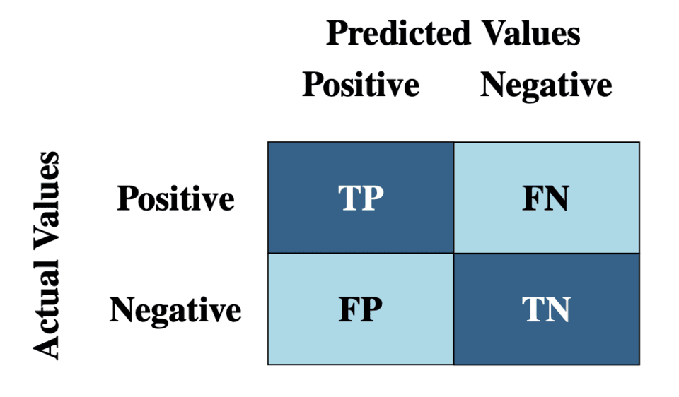
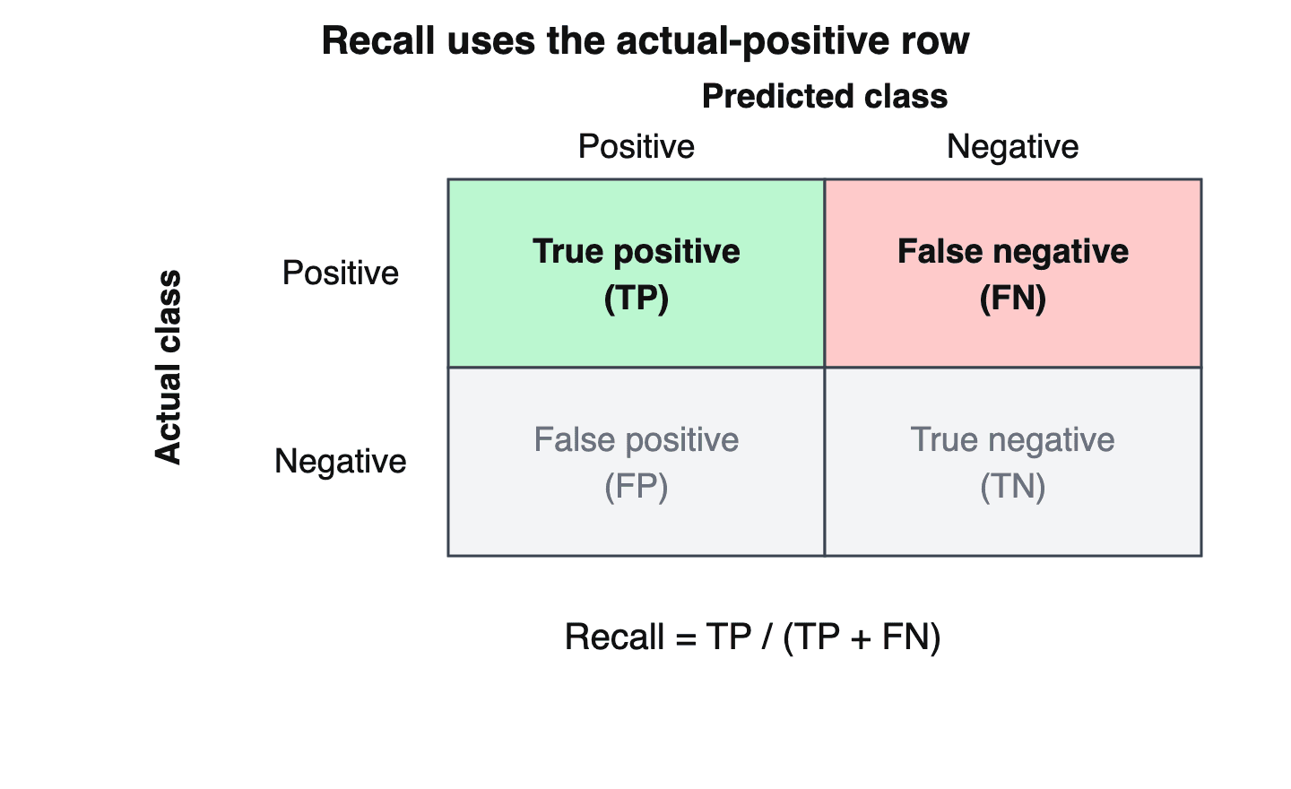
For a binary classifier evaluated on $n$ examples, the confusion matrix records four counts:[2]
| Predicted positive | Predicted negative | |
|---|---|---|
| Actual positive | True positives (TP) | False negatives (FN) |
| Actual negative | False positives (FP) | True negatives (TN) |
The coefficient is defined as:[2][3]
The numerator compares the product of the two kinds of correct prediction with the product of the two kinds of error. The factors under the square root are the numbers of predicted positives, actual positives, actual negatives and predicted negatives, which are the marginal totals that enter the variances of the predicted and actual label vectors.[5]
Range and interpretation
MCC reaches +1 for a perfect prediction (FP = FN = 0) and -1 for a complete inversion of the labels (TP = TN = 0).[5] Chicco and Jurman note that 0 is the expected value for a classifier that assigns each label by tossing a coin.[2] Formally, MCC is 0 exactly when TP·TN = FP·FN. For any non-degenerate dataset this is the same as the true positive rate equalling the false positive rate, so the classifier sits on the diagonal of ROC space; the sign of MCC is positive when the true positive rate exceeds the false positive rate and negative when it falls below it.[5] Jesús S. Aguilar-Ruiz therefore argues that a zero score should be read as "no linear correlation between prediction and truth" rather than as proof that predictions are random: a deterministic classifier with TP = 99, FN = 1, FP = 99 and TN = 1 also scores exactly 0.[5]
To put MCC on the same [0, 1] scale as most other rates, it is sometimes normalized as nMCC = (MCC + 1)/2, a linear map under which 0.5 is the coin-tossing value.[2][14]
Equivalent forms
Matthews himself defined the coefficient as the ordinary product-moment correlation between a prediction vector $P$ and an observation vector $S$, following the treatment in R. A. Fisher's statistics textbook. For step functions taking only the values 0 and 1 he rewrote it as[5]
where $p$ is the number of residues both predicted and observed to be in the structure (the true positives), $\bar{S}$ is the fraction of positive observations and $\bar{P}$ is the fraction of positive predictions.[5] Expanding the Pearson correlation of two binary vectors in terms of the four counts gives the modern formula above, which is why the CoLA authors describe MCC as "a special case of Pearson's r for Boolean variables".[5][13]
Several other identities are used in the literature:
| Form | Expression | Source |
|---|---|---|
| Informedness and markedness | $\text{MCC} = \pm\sqrt{\text{BM}\cdot\text{MK}}$, where bookmaker informedness BM = TPR + TNR - 1 and markedness MK = PPV + NPV - 1 | [6][7] |
| Four basic rates and their complements | $\sqrt{\text{PPV}\cdot\text{TPR}\cdot\text{TNR}\cdot\text{NPV}} - \sqrt{\text{FDR}\cdot\text{FNR}\cdot\text{FPR}\cdot\text{FOR}}$ | [7] |
| Chi-squared statistic | $\chi^2 = n \cdot \text{MCC}^2$ for a 2x2 table | [5] |
| Normalized MCC | $\text{nMCC} = (\text{MCC}+1)/2$ | [2] |
Here TPR is recall (sensitivity), TNR is specificity, PPV is precision, NPV is the negative predictive value, and FDR, FNR, FPR and FOR are the corresponding error rates.[2][7] David Powers's 2011 paper on informedness and markedness sets out this geometric-mean form, noting that Perruchet and Peereman had already described the geometric mean of the two underlying regression coefficients as a dichotomous form of the Pearson correlation.[6] Chicco, Tötsch and Jurman read it as saying that MCC is high only when the classifier is well informed (high BM) and the actual class is well marked by the predicted label (high MK).[7]
Undefined cases
The formula divides by zero whenever a whole row or a whole column of the confusion matrix is zero, for example when a classifier predicts the same class for every example.[2] Chicco and Jurman fill these gaps with a limit argument. If only one cell is non-zero, every example belongs to one class and is either correctly classified (MCC = +1) or misclassified (MCC = -1). In the four remaining cases, replacing the zero entries with a small value $\varepsilon$ and letting $\varepsilon \to 0$ gives MCC = 0, so the trivial classifier that always predicts the majority class scores 0.[2] scikit-learn takes a simpler route: its matthews_corrcoef function returns 0.0 whenever the denominator is zero.[8]
History
Antecedents
The coefficient is older than its name. In a 2026 survey titled "The Matthews Correlation Coefficient: Fifty years", Aguilar-Ruiz traces an expression structurally similar to the modern formula to Karl Pearson's 1900 treatment of the correlation in a fourfold (2x2) table, and describes the phi coefficient as the binary analogue of Pearson correlation for such tables.[5] The same survey points to M. H. Doolittle's 1884 work on the verification of predictions, whose association ratio is exactly the square of MCC.[5] Chicco and Jurman likewise describe MCC as a special case of the phi coefficient.[2]
Matthews (1975)
Brian W. Matthews, a structural biologist who is now an emeritus biochemist and biophysicist at the University of Oregon, published "Comparison of the predicted and observed secondary structure of T4 phage lysozyme" in Biochimica et Biophysica Acta on 20 October 1975.[1][5] The paper compared secondary-structure predictions that several investigators had made from the amino acid sequence with the structure determined by X-ray crystallography.[1] Matthews classified each residue into four categories (predicted and observed helical, predicted and observed non-helical, underpredicted, and overpredicted), judged some earlier agreement measures unsuitable, and used the correlation coefficient instead.[5] For eleven different helix predictions the coefficient ranged from 0.14 to 0.42; predictions of beta-sheet regions and turns were generally less accurate, and in several cases agreement was no better than would be expected for a random selection of residues.[1]
Adoption
From 1975 until the end of the 1990s the coefficient was used mainly in structural biology, where it became a standard way to benchmark protein secondary-structure predictors, including the early neural network methods of the late 1980s and 1990s.[5] According to Aguilar-Ruiz, its first appearance in a computer science journal was a 1993 Machine Learning article by Cost and Salzberg, where it again scored protein secondary-structure predictions.[5] Its wider popularity dates from a 2000 Bioinformatics overview by Baldi, Brunak, Chauvin, Andersen and Nielsen, which compared accuracy measures ranging from raw percentages to correlation coefficients and information-theoretic quantities, and derived learning algorithms that directly optimize the correlation coefficient.[9][5]
| Year | Development | Ref. |
|---|---|---|
| 1975 | Matthews scores protein secondary-structure predictions for T4 phage lysozyme | [1] |
| 1993 | First use in a computer science journal (Cost and Salzberg, Machine Learning) | [5] |
| 2000 | Baldi et al. review prediction-accuracy measures and optimize the correlation coefficient directly | [9] |
| 2004 | Gorodkin proposes the K-category generalization $R_K$ | [10] |
| 2010 | The MAQC-II consortium reports the performance of more than 30,000 models by MCC | [11] |
| 2018 | GLUE adopts MCC for CoLA and $R_3$ for its diagnostic set | [12] |
| 2020 | Chicco and Jurman argue that MCC should be preferred to accuracy and F1 | [2] |
| 2023 | Chicco and Jurman argue that MCC should replace ROC AUC as the standard binary metric | [14] |
| 2026 | Aguilar-Ruiz publishes a fifty-year survey of the coefficient | [5] |
Properties
MCC uses all four cells of the confusion matrix explicitly, unlike the F1 score or sensitivity.[5] It is symmetric: swapping which class is called positive leaves its value unchanged, whereas the F1 score and precision change.[2][5] Chicco and Jurman stress a further property: a high MCC is possible only when sensitivity, specificity, precision and negative predictive value are all high, and in their words the MCC "does not lie" on this point.[14] The same authors note the cost of this summary: a low MCC says that a classifier failed but not why, so they recommend reporting the four basic rates alongside it.[14]
MCC and the F1 score agree in many cases but can diverge widely. Chicco and Jurman show that for a given F1 value $\phi$ the MCC can lie roughly anywhere in $[\phi - 1, \phi]$, and that much of this spread comes from F1 ignoring true negatives.[2] Computing all possible confusion matrices for a dataset of 1,000 samples, they found a Pearson correlation of about 0.92 between MCC and accuracy but only about 0.78 between MCC and F1.[2]
Comparison with accuracy and F1 on imbalanced data
Accuracy can look excellent on a class-imbalanced dataset simply because the majority class dominates the count, and the F1 score ignores true negatives and depends on which class is labelled positive.[2] Chicco and Jurman's 2020 paper in BMC Genomics illustrates the difference with six synthetic confusion matrices for datasets of 100 examples:[2]
| Use case | Positives / negatives | TP | FN | TN | FP | Accuracy | F1 | MCC |
|---|---|---|---|---|---|---|---|---|
| A1 | 91 / 9 | 90 | 1 | 0 | 9 | 0.90 | 0.95 | -0.03 |
| A2 | 75 / 25 | 5 | 70 | 19 | 6 | 0.24 | 0.12 | -0.24 |
| B1 | 50 / 50 | 47 | 3 | 5 | 45 | 0.52 | 0.66 | +0.07 |
| B2 | 50 / 50 | 10 | 40 | 46 | 4 | 0.56 | 0.31 | +0.17 |
| C1 | 10 / 90 | 9 | 1 | 1 | 89 | 0.10 | 0.17 | -0.19 |
| C2 | 11 / 89 | 2 | 9 | 88 | 1 | 0.90 | 0.29 | +0.31 |
In use case A1 the classifier labels almost everything positive and identifies none of the nine negatives, yet accuracy (0.90) and F1 (0.95) are close to their maximum; only MCC, at -0.03, is close to zero and signals that the classifier performed poorly.[2] In B1, F1 alone is misleadingly high, and in C2 accuracy alone is misleadingly high.[2] The authors conclude that MCC was the only one of the three rates that flagged the problem in all six cases, and suggest that all researchers working with confusion matrices evaluate binary predictions with MCC instead of accuracy or F1.[2]
The paper also ranks five classifiers on a public colon cancer gene-expression dataset (62 patients, 40 with cancer). Ranked by MCC, gradient boosting comes first (MCC +0.55); ranked by F1 or by accuracy, k-nearest neighbors comes first, even though its true negative rate (0.52) is well below that of gradient boosting (0.69).[2]
Similar arguments have been made in other fields. A 2020 review of software defect prediction studies by Yao and Shepperd collected 4,017 pairwise comparisons from 8 studies that reported both F1 and MCC, and found that the direction of the comparison changed in 23% of cases when MCC was used; the authors called for F1 to be deprecated in that field.[23] The CoLA authors describe MCC in a footnote as an evaluation metric for unbalanced binary classifiers: on average, "any two unrelated distributions will have an MCC of 0, regardless of class imbalance", whereas accuracy and F1 favour classifiers with a majority-class bias.[13]
Chicco and Jurman do not claim that MCC suits every goal. When correctly classifying positive cases matters more than negative ones, they write, the F1 score or the Fowlkes-Mallows index can be more appropriate, although they still recommend reporting MCC.[14]
Comparison with other measures
| Measure | Relationship to MCC | Source |
|---|---|---|
| ROC AUC | Threshold-free. Chicco and Jurman argue that it says nothing about precision or negative predictive value, that one (sensitivity, specificity) pair can cover a broad range of MCC values, and that a high MCC always corresponds to a high ROC AUC but not the reverse. | [14] |
| Balanced accuracy and bookmaker informedness | BA = (TPR + TNR)/2 and BM = TPR + TNR - 1 carry the same information, and both describe the classifier independently of the test dataset; BM is identical to Youden's J statistic. | [7] |
| Markedness | MK = PPV + NPV - 1; MCC is the geometric mean of BM and MK. | [6][7] |
| Cohen's kappa | Delgado and Tibau found kappa and MCC correlated in most situations, but in some unbalanced cases kappa gave a worse classifier a higher score. | [16] |
| Brier score | A probability-based score; Chicco, Warrens and Jurman report use cases in which MCC gives the more informative result. | [15] |
| Confusion entropy (CEN) | Jurman, Riccadonna and Furlanello showed a strong monotone relation between CEN and multiclass MCC. | [17] |
In their 2021 comparison with balanced accuracy, bookmaker informedness and markedness, Chicco, Tötsch and Jurman identified three situations in which bookmaker informedness is the better choice: when the prevalence in the test data does not represent the population of interest, when comparing classifiers across different datasets, and when asking whether a classifier performs better than random guessing. Outside those cases they recommend MCC as the standard measure.[7]
Criticism and limitations
Dependence on class prevalence
MCC is often described as "balanced", and the scikit-learn documentation says it "can be used even if the classes are of very different sizes".[3] Several authors have tested how far that description holds. Aguilar-Ruiz proves that MCC is unchanged only when both classes are rescaled by the same factor. In his example, a classifier with a true positive rate of 2/3 and a true negative rate of 3/4 scores 0.417 on a test set with 3 positives and 4 negatives, but only 0.305 when the negatives are multiplied by five, although both rates are unchanged.[5] He notes that some recent publications still state that MCC is invariant to class imbalance.[5]
Chicco, Tötsch and Jurman also describe MCC as biased by class imbalance. In their use case UC1 a classifier with a true positive rate of 0.99 and a true negative rate of 0.95 is applied to 100,001 examples of which 101 are positive (TP = 100, FN = 1, FP = 5,000, TN = 94,900). Its MCC is 0.136 while its bookmaker informedness is 0.94. They read the low MCC as a warning that at least one basic rate is low, here precision (about 0.02), but conclude that MCC "in general does not tell us if a classifier performs similarly to random guessing because it is biased by class imbalance".[7]
Qiuming Zhu, writing in Pattern Recognition Letters in 2020, went further, reporting that MCC "deteriorates seriously" when the classes are imbalanced and concluding that it is not suitable for measuring classification accuracy on imbalanced datasets.[18] Hajo Holzmann and Bernhard Klar analyse the problem from the side of the optimal classifier. In a preprint last revised in October 2026, they show that as the proportion of the minority class tends to zero, the true positive rate of the Bayes classifier under MCC (and under Cohen's kappa, the F-score and the Jaccard coefficient) becomes very small or tends to zero, so these metrics can favour classifiers that ignore the minority class. They propose robustified versions of MCC, Cohen's kappa and the F-score with a tuning parameter that sets how much robustness to class imbalance the metric provides.[19]
Giles Foody, writing in PLOS ONE in 2023, questioned the claim that a high MCC can only come from a classifier that performs well on both classes. In his simulations, which used realistic values of data quality for applications such as remote sensing, variation in prevalence and an imperfect reference standard caused the apparent MCC to be substantially under- or over-estimated, and a high apparent MCC arose from an unquestionably poor classification. He concluded that, as with some other accuracy metrics, the utility of MCC may be overstated and apparent values should be interpreted with caution.[28]
Other limitations
Like accuracy and F1, MCC is computed from a confusion matrix at one classification threshold.[2] Chicco and Jurman list this heuristic cut-off (usually 0.5) and the undefined cases as its limitations.[14] In their 2020 paper they also note that in extreme situations MCC can be undefined or fluctuate strongly.[2]
Statistical uncertainty
A single MCC value is a point estimate. Itaya, Tamura, Hayashi and Yamamoto observed that studies often compare MCC point estimates without assessing their statistical significance, and developed asymptotic confidence intervals for one MCC and for the difference between two MCCs in paired designs; a follow-up extends this to macro- and micro-averaged multiclass MCC.[20][21] Aguilar-Ruiz warns that the familiar Fisher z-transformation assumes bivariate normality, which binary labels do not satisfy, and can give intervals that are too narrow. For an MCC of 0.65 on 1,000 examples, his Fisher interval is [0.613, 0.684], while inverting a likelihood-ratio (chi-squared) test gives the wider [0.588, 0.712]; for small or highly skewed samples he suggests the bootstrap.[5]
Multiclass extension
In 2004 Jan Gorodkin introduced $R_K$, a correlation coefficient for comparing two assignments into $K$ categories. He was motivated by the practice of forcing multi-category problems into two categories (one class against the rest), which loses information, and applied it to RNA secondary-structure prediction with an extra "unknown" category.[10] scikit-learn computes the multiclass MCC from a $K \times K$ confusion matrix $C$ as[4]
where $t_k$ is the number of times class $k$ truly occurred, $p_k$ the number of times it was predicted, $c$ the total number of correct predictions and $s$ the total number of samples. The maximum is still +1, but the minimum lies somewhere between -1 and 0 depending on the number of classes and the distribution of the true labels.[4]
GLUE uses $R_3$, the three-class case, for its natural language inference diagnostic set because that set's class distribution is unbalanced.[12] Jurman and colleagues showed that multiclass MCC is strongly and monotonically related to the confusion entropy measure.[17] Petre Stoica and Prabhu Babu argue that $R_K$ and multivariate Pearson correlation metrics do not always signal poor results decisively when they should, and propose enhanced multiclass metrics.[22] Tamura and colleagues note that macro- and micro-averaged multiclass MCCs have been used without clear definitions, and give formal definitions together with confidence intervals.[21]
Use in machine learning
Benchmarks and evaluation studies
The GLUE benchmark reports MCC for CoLA, the Corpus of Linguistic Acceptability, following the dataset's authors; GLUE describes the metric as one that "evaluates performance on unbalanced binary classification".[12] CoLA contains 10,657 English sentences from the linguistics literature labelled as grammatical or ungrammatical. In the original study, individual human annotators agreed with the CoLA labels with an average MCC of 0.697, and the majority vote of the annotators reached 0.713.[13]
In genomics, the MicroArray Quality Control (MAQC-II) study had 36 independent teams build more than 30,000 predictive models on six microarray datasets for 13 endpoints. The study reported performance by MCC "because it is informative when the distribution of the two classes in a data set is highly skewed and because it is simple to calculate and was available for all models". The easiest endpoints reached a mean MCC above 0.7, while the negative-control endpoints stayed near 0, as expected.[11] Chicco and Jurman cite the MAQC-II and SEQC projects as cases in which the US Food and Drug Administration used MCC as the main evaluation measure.[2]
As a training objective
Baldi and colleagues already derived learning algorithms that optimize the correlation coefficient directly in 2000.[9] In 2017 Sabri Boughorbel, Fethi Jarray and Mohammed El-Anbari derived an optimal Bayes classifier for the MCC metric aimed at imbalanced biomedical data; on 64 datasets it performed close to an imbalanced support vector machine while being simpler and more efficient.[24] In image segmentation, Kumar Abhishek and Ghassan Hamarneh proposed an MCC-based loss function for skin lesion segmentation, noting that the popular Dice loss does not penalize misclassified background pixels. Models trained with it improved the mean Jaccard index over Dice loss by 11.25%, 4.87% and 0.76% on three skin lesion datasets.[25]
Software
| Library | Interface | Notes | Source |
|---|---|---|---|
| scikit-learn | sklearn.metrics.matthews_corrcoef(y_true, y_pred, *, sample_weight=None) | Binary and multiclass labels; returns 0.0 when the denominator is zero | [3][8] |
| Hugging Face Evaluate | evaluate.load("matthews_correlation") | Takes predictions and references; optional per-label or macro average in the multilabel case | [26] |
| TorchMetrics (PyTorch) | MatthewsCorrCoef(task=...) | Binary, multiclass and multilabel variants | [27] |
The scikit-learn documentation gives a minimal example:[3]
>>> from sklearn.metrics import matthews_corrcoef
>>> y_true = [+1, +1, +1, -1]
>>> y_pred = [+1, -1, +1, +1]
>>> matthews_corrcoef(y_true, y_pred)
-0.33
Continue reading
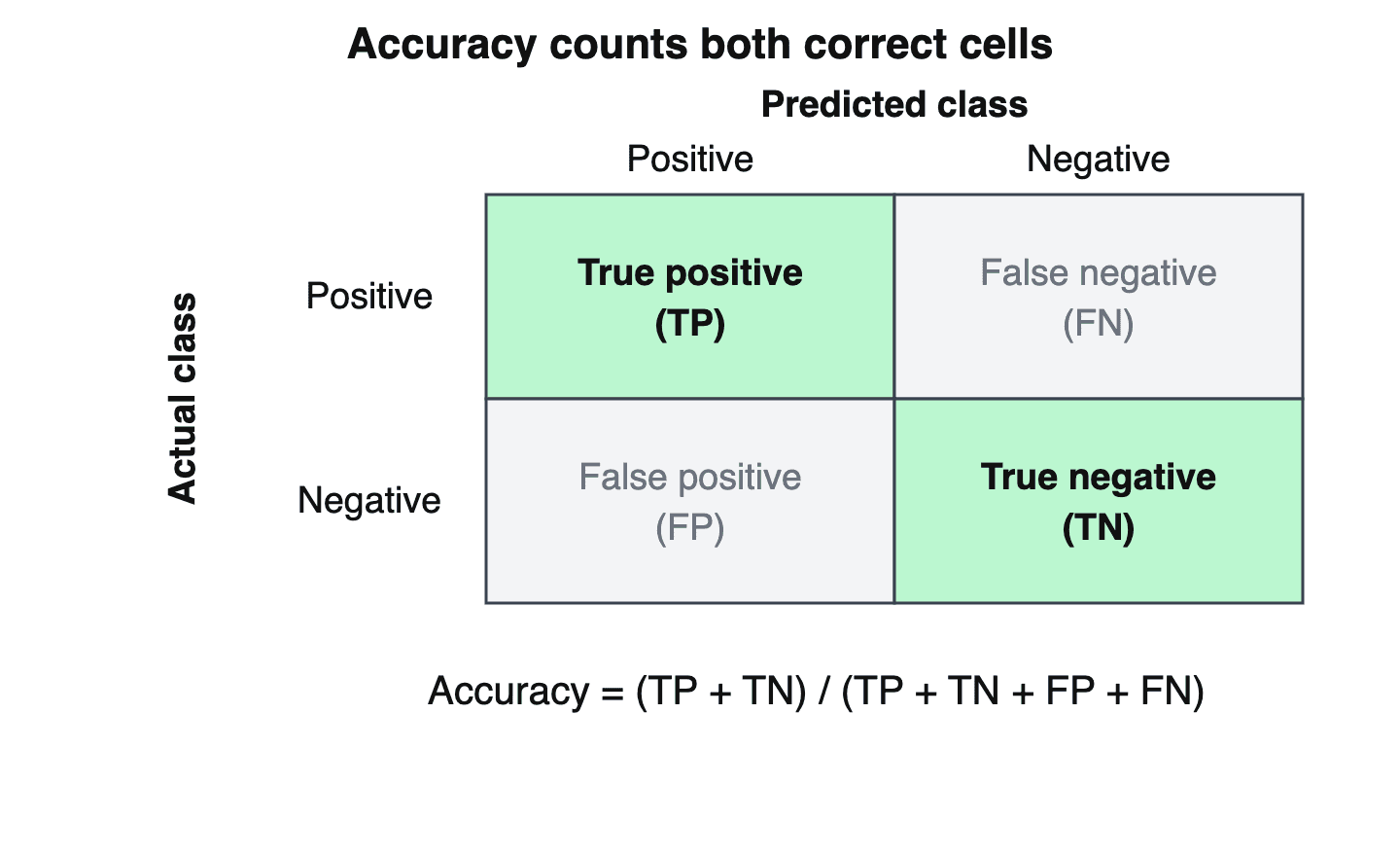
- AccuracyAccuracy is a classification metric that measures the fraction of predictions a model gets right: the number of correct predictions divided by the total number of predictions.Mentioned 18 times above
- Confusion MatrixA confusion matrix is a table that summarizes the performance of a classification model by tabulating its predicted class labels against the actual class labels, with correct predictions on the diagonal and…Mentioned 6 times above
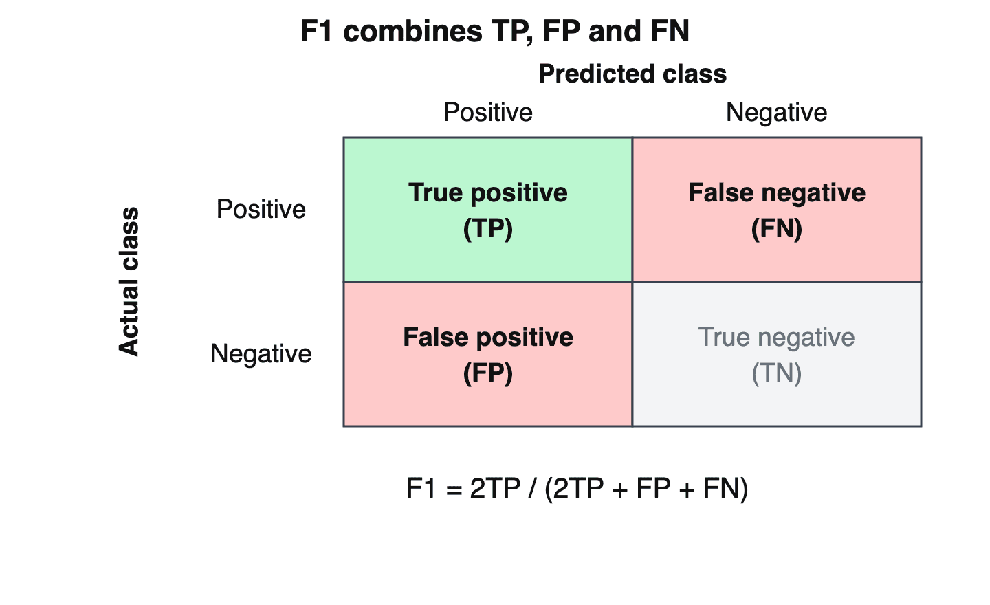
- F1 scoreThe F1 score (also written as F1-score, F-score, or F-measure) is the harmonic mean of precision and recall.Mentioned 6 times above
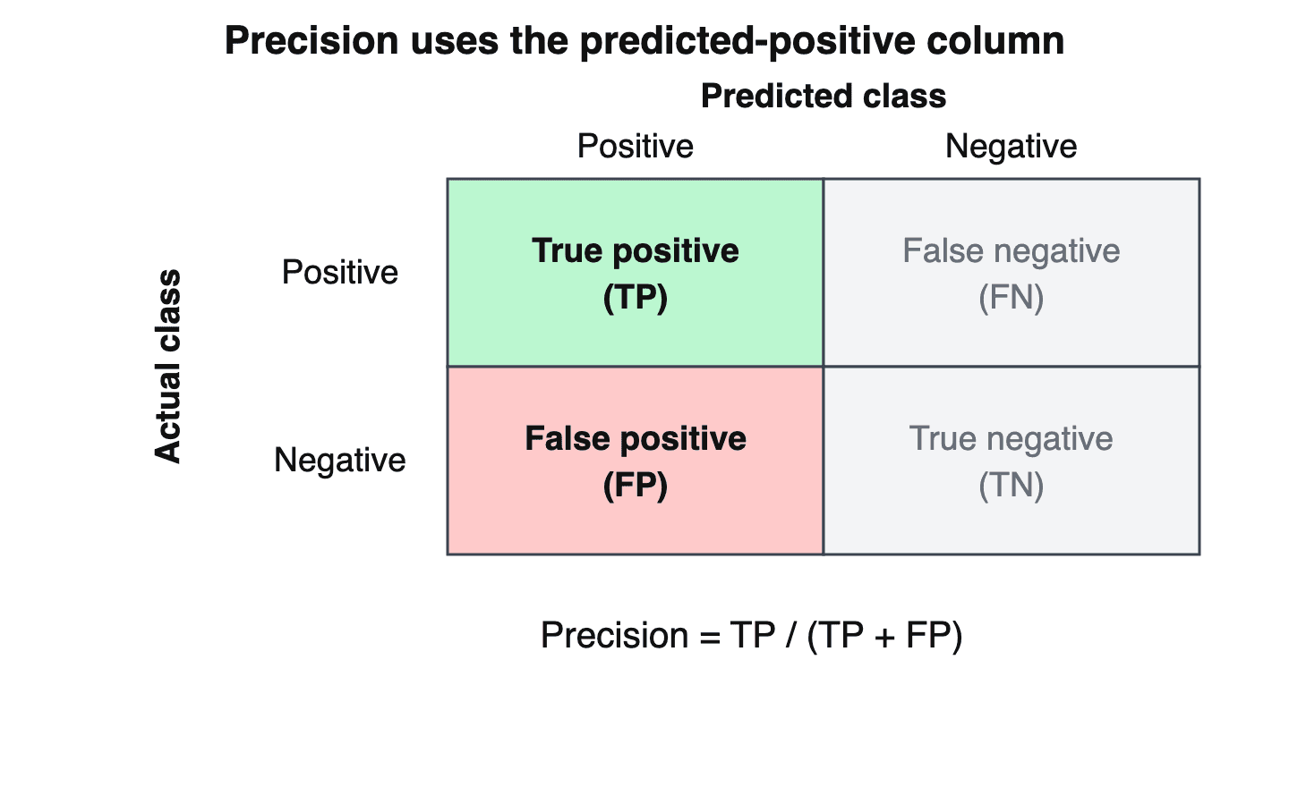
- PrecisionPrecision is a classification metric defined as the fraction of positive predictions that are correct: Precision = TP / (TP + FP), where TP is the number of true positives and FP is the number of false…Mentioned 5 times above
- ROC (Receiver Operating Characteristic) CurveA Receiver Operating Characteristic (ROC) curve is a graph that measures how well a binary classification system separates two classes by plotting its true positive rate (TPR, also called sensitivity or…Mentioned 4 times above
- Recall (metric)Recall is a classification and retrieval metric that measures the proportion of actual positive instances a model correctly identifies, defined as TP / (TP + FN)Listed in See also
More from See also
More to read
References
- ^1 ^2 ^3 ^4 ^5Matthews, B. W. "Comparison of the predicted and observed secondary structure of T4 phage lysozyme". Biochimica et Biophysica Acta (BBA) - Protein Structure, 405(2), 442-451, October 1975. pubmed.ncbi.nlm.nih.gov/1180967
- ^1 ^2 ^3 ^4 ^5 ^6 ^7 ^8 ^9 ^10 ^11 ^12 ^13 ^14 ^15 ^16 ^17 ^18 ^19 ^20 ^21 ^22 ^23 ^24 ^25 ^26Chicco, D., & Jurman, G. "The advantages of the Matthews correlation coefficient (MCC) over F1 score and accuracy in binary classification evaluation". BMC Genomics, 21, 6, 2020. doi.org/...s12864-019-6413-7
- ^1 ^2 ^3 ^4 ^5scikit-learn developers. "matthews_corrcoef". scikit-learn 1.9.1 documentation. scikit-learn.org/...earn.metrics.matthews_corrcoef
- ^1 ^2scikit-learn developers. "3.4. Metrics and scoring: quantifying the quality of predictions" (section 3.4.4.13, Matthews correlation coefficient). scikit-learn 1.9.1 documentation. scikit-learn.org/...model_evaluation
- ^1 ^2 ^3 ^4 ^5 ^6 ^7 ^8 ^9 ^10 ^11 ^12 ^13 ^14 ^15 ^16 ^17 ^18 ^19 ^20 ^21 ^22 ^23 ^24 ^25 ^26 ^27Aguilar-Ruiz, J. S. "The Matthews Correlation Coefficient: Fifty years". arXiv:2611.08799, 5 November 2026. arxiv.org/...2611.08799
- ^1 ^2 ^3Powers, D. M. W. "Evaluation: From Precision, Recall and F-Measure to ROC, Informedness, Markedness and Correlation". International Journal of Machine Learning Technology, 2(1), 37-63, 2011 (arXiv:2010.16061). arxiv.org/...2010.16061
- ^1 ^2 ^3 ^4 ^5 ^6 ^7 ^8Chicco, D., Tötsch, N., & Jurman, G. "The Matthews correlation coefficient (MCC) is more reliable than balanced accuracy, bookmaker informedness, and markedness in two-class confusion matrix evaluation". BioData Mining, 14, 13, 2021. doi.org/...s13040-021-00244-z
- ^1 ^2scikit-learn developers. "sklearn/metrics/_classification.py" (matthews_corrcoef source, tag 1.9.1). GitHub. github.com/..._classification.py
- ^1 ^2 ^3Baldi, P., Brunak, S., Chauvin, Y., Andersen, C. A. F., & Nielsen, H. "Assessing the accuracy of prediction algorithms for classification: an overview". Bioinformatics, 16(5), 412-424, May 2000. doi.org/...16.5.412
- ^1 ^2Gorodkin, J. "Comparing two K-category assignments by a K-category correlation coefficient". Computational Biology and Chemistry, 28(5-6), 367-374, December 2004. doi.org/...j.compbiolchem.2004.09.006
- ^1 ^2Shi, L., Campbell, G., Jones, W. D., et al. (MAQC Consortium). "The MicroArray Quality Control (MAQC)-II study of common practices for the development and validation of microarray-based predictive models". Nature Biotechnology, 28(8), 827-838, August 2010. doi.org/...nbt.1665
- ^1 ^2 ^3 ^4Wang, A., Singh, A., Michael, J., Hill, F., Levy, O., & Bowman, S. R. "GLUE: A Multi-Task Benchmark and Analysis Platform for Natural Language Understanding". ICLR 2019 (arXiv:1804.07461). arxiv.org/...1804.07461
- ^1 ^2 ^3Warstadt, A., Singh, A., & Bowman, S. R. "Neural Network Acceptability Judgments". Transactions of the Association for Computational Linguistics, 7, 625-641, 2019 (arXiv:1805.12471). arxiv.org/...1805.12471
- ^1 ^2 ^3 ^4 ^5 ^6 ^7Chicco, D., & Jurman, G. "The Matthews correlation coefficient (MCC) should replace the ROC AUC as the standard metric for assessing binary classification". BioData Mining, 16, 4, February 2023. doi.org/...s13040-023-00322-4
- ^Chicco, D., Warrens, M. J., & Jurman, G. "The Matthews Correlation Coefficient (MCC) is More Informative Than Cohen's Kappa and Brier Score in Binary Classification Assessment". IEEE Access, 9, 78368-78381, 2021. doi.org/...ACCESS.2021.3084050
- ^Delgado, R., & Tibau, X.-A. "Why Cohen's Kappa should be avoided as performance measure in classification". PLOS ONE, 14(9), e0222916, September 2019. doi.org/...journal.pone.0222916
- ^1 ^2Jurman, G., Riccadonna, S., & Furlanello, C. "A Comparison of MCC and CEN Error Measures in Multi-Class Prediction". PLoS ONE, 7(8), e41882, August 2012. doi.org/...journal.pone.0041882
- ^1 ^2Zhu, Q. "On the performance of Matthews correlation coefficient (MCC) for imbalanced dataset". Pattern Recognition Letters, 136, 71-80, August 2020. doi.org/...j.patrec.2020.03.030
- ^1 ^2Holzmann, H., & Klar, B. "Robust performance metrics for imbalanced classification problems". arXiv:2404.07661 (version 3, 29 October 2026). arxiv.org/...2404.07661
- ^Itaya, Y., Tamura, J., Hayashi, K., & Yamamoto, K. "Asymptotic Properties of Matthews Correlation Coefficient". Statistics in Medicine, 44(1-2), e10303, 2025. doi.org/...sim.10303
- ^1 ^2Tamura, J., Itaya, Y., Hayashi, K., & Yamamoto, K. "Statistical inference of the Matthews correlation coefficient for multiclass classification". Journal of Applied Statistics, 2026 (arXiv:2503.06450). arxiv.org/...2503.06450
- ^Stoica, P., & Babu, P. "Pearson-Matthews correlation coefficients for binary and multinary classification". Signal Processing, 222, 109511, 2024 (arXiv:2305.05974). doi.org/...j.sigpro.2024.109511
- ^Yao, J., & Shepperd, M. "Assessing software defection prediction performance: why using the Matthews correlation coefficient matters". Proceedings of the Evaluation and Assessment in Software Engineering (EASE 2020), 120-129, April 2020 (arXiv:2003.01182). arxiv.org/...2003.01182
- ^Boughorbel, S., Jarray, F., & El-Anbari, M. "Optimal classifier for imbalanced data using Matthews Correlation Coefficient metric". PLOS ONE, 12(6), e0177678, June 2017. doi.org/...journal.pone.0177678
- ^Abhishek, K., & Hamarneh, G. "Matthews Correlation Coefficient Loss for Deep Convolutional Networks: Application to Skin Lesion Segmentation". 2021 IEEE 18th International Symposium on Biomedical Imaging (ISBI), 225-229, 2021 (arXiv:2010.13454). arxiv.org/...2010.13454
- ^Hugging Face. "Metric Card for Matthews Correlation Coefficient". Evaluate library, GitHub. github.com/...README.md
- ^Lightning AI. "Matthews Correlation Coefficient". TorchMetrics 1.9.0 documentation. lightning.ai/...matthews_corr_coef
- ^Foody, G. M. "Challenges in the real world use of classification accuracy metrics: From recall and precision to the Matthews correlation coefficient". PLOS ONE, 18(10), e0291908, October 2023. doi.org/...journal.pone.0291908
Improve this article
Add missing citations, update stale details, or write a clearer explanation. Anyone can edit: changes go live when you publish, and every edit is checked by an editor.
1 revision · v1 · 4,395 words · full history
Fact-checks are independent of edits: a reviewer re-verifies the article against its sources and stamps the date. How we verify
Research and drafting on this wiki are AI-assisted, under named human editorial standards. How AI is used here
Reviewer note: Independent fact-check before publication on November 18, 2026: 96 claims checked against 31 cited and independent sources; 0 material and 4 minor corrections applied before publication.
Cite this page: AI Wiki. "Matthews Correlation Coefficient." aiwiki.ai, updated 18 Nov 2026, fact-checked 18 Nov 2026. CC BY 4.0. https://aiwiki.ai/wiki/matthews_correlation_coefficient