

Probability distribution
A probability distribution is a description of how likely a random variable, or a set of random variables, is to take on each of its possible values [1]. A distribution over a discrete variable is usually written as a probability mass function (PMF), and a distribution over a continuous variable as a probability density function (PDF); both can be summarized by a cumulative distribution function (CDF) [3]. Machine learning relies on them throughout. Training data are modeled as samples from an unknown data-generating distribution, most neural networks are trained by maximum likelihood so that the distribution they define matches the data [4][5], and generative models try to represent and sample from complex distributions over data such as images [15][18].
Definition
Random variables and the axioms of probability
A random variable is a variable that can take on different values randomly. On its own it only lists the states that are possible; it has to be paired with a probability distribution that says how likely each state is [1]. A discrete random variable has a finite or countably infinite number of states, which need not be numbers at all (they can be named categories), while a continuous random variable takes real values [1].
The standard mathematical foundation is the axiomatization in A. N. Kolmogorov's Foundations of the Theory of Probability (1933). A probability function assigns each event $A$ a number with $P(A) \ge 0$, gives the whole outcome space $\Omega$ probability $P(\Omega) = 1$, and is additive over disjoint events; Kolmogorov strengthened additivity from finite to countable unions, a choice that philosophers of probability still debate [2].
Discrete distributions: the probability mass function
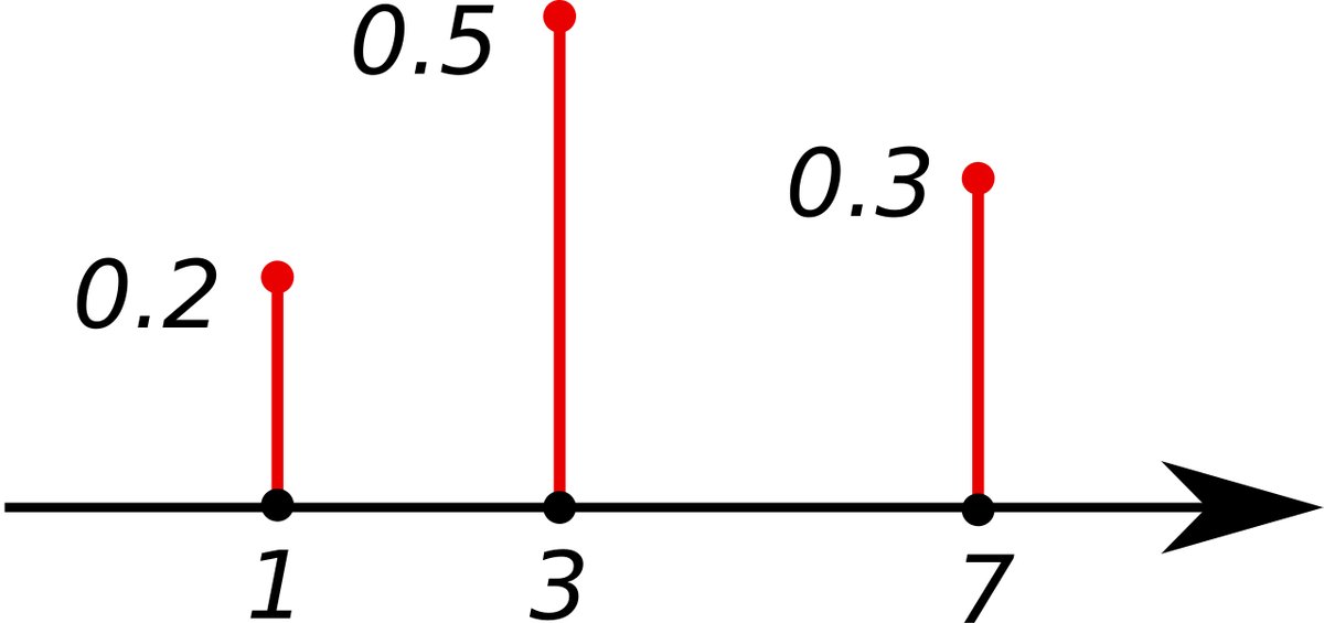
For a discrete variable $x$, a PMF $P$ maps each state to the probability that the variable takes that state. To be a valid PMF, $P$ must be defined on every possible state, must satisfy $0 \le P(x) \le 1$ for each state, and must be normalized so that $\sum_x P(x) = 1$ [1]. A uniform distribution over $k$ states, for example, sets $P(x = x_i) = 1/k$ for every $i$, which sums to $k/k = 1$ [1]. A distribution over several variables at once, $P(x, y)$, is called a joint probability distribution [1].
Continuous distributions: the probability density function
For a continuous variable, a PDF $p$ must be non-negative everywhere and must integrate to 1, but unlike a PMF it is not required to stay below 1 [1]. The density at a point is not a probability. Instead, the probability of landing in a tiny region of volume $\delta x$ is approximately $p(x),\delta x$, and the probability that $x$ falls in an interval $[a, b]$ is the integral of $p(x)$ over that interval [1]. The uniform density on $[a, b]$, for instance, equals $1/(b - a)$ inside the interval and 0 outside it [1].
Cumulative distribution function and quantiles
The cumulative distribution function gives the probability that a variable is less than or equal to a value: $F(x) = \Pr[X \le x]$. For a continuous distribution it is the integral of the density from $-\infty$ to $x$, and for a discrete distribution it is the sum of the PMF over all values up to $x$ [3]. Several related functions are defined from it [3]:
| Function | Definition |
|---|---|
| Cumulative distribution function | $F(x) = \Pr[X \le x]$ |
| Percent point (quantile) function | The inverse of the CDF |
| Survival function | $S(x) = \Pr[X > x] = 1 - F(x)$ |
| Hazard function | $h(x) = f(x) / S(x)$, the density divided by the survival function |
Joint, marginal and conditional distributions
Most models in machine learning involve many variables, so a handful of rules for moving between joint and partial descriptions are used constantly [1]:
- Marginalization (sum rule). The distribution over a subset of variables is found by summing out the others, $P(x) = \sum_y P(x, y)$, or by integrating them out in the continuous case. The name comes from writing the joint table on paper and recording row sums in the margin [1].
- Conditional probability. $P(y \mid x) = P(y, x) / P(x)$, defined only when $P(x) > 0$ [1]. Goodfellow, Bengio and Courville stress that conditioning is not the same as intervening: the probability that a person is from Germany given that they speak German is high, but teaching someone German does not change where they come from. Questions about actions belong to causal modeling [1].
- Chain rule (product rule). Any joint distribution factorizes into one-variable conditionals, $P(x^{(1)}, \ldots, x^{(n)}) = P(x^{(1)}) \prod_{i=2}^{n} P(x^{(i)} \mid x^{(1)}, \ldots, x^{(i-1)})$ [1].
- Independence. Two variables are independent when their joint distribution is the product of their marginals, and conditionally independent given $z$ when that factorization holds for every value of $z$ [1].
- Bayes' rule. $P(x \mid y) = P(x) P(y \mid x) / P(y)$, where the denominator can be computed as $\sum_x P(y \mid x) P(x)$. The rule is named after Thomas Bayes, who discovered a special case; Pierre-Simon Laplace independently found the general version [1]. The same identity is known as Bayes' theorem, and it is the basis of Bayesian inference.
Factorizing a joint distribution into small factors is the idea behind structured probabilistic models, also called graphical models, which come in directed and undirected forms. Such factorizations can greatly reduce the number of parameters needed to describe a distribution [1].
Expectation, variance and covariance
The expectation of a function $f(x)$ under a distribution is its average value when $x$ is drawn from that distribution: $\mathbb{E}_{x \sim P}[f(x)] = \sum_x P(x) f(x)$ for discrete variables and $\int p(x) f(x),dx$ for continuous ones. Expectation is linear [1]. The variance, $\mathrm{Var}(f(x)) = \mathbb{E}[(f(x) - \mathbb{E}[f(x)])^2]$, measures how much values spread around their mean, and its square root is the standard deviation [1]. Covariance measures how two quantities vary together. Independent variables have zero covariance, but zero covariance does not imply independence, because covariance only detects linear dependence: if $x$ is uniform on $[-1, 1]$ and $y = sx$ for a random sign $s$, then $x$ and $y$ are dependent yet have zero covariance [1].
What probabilities mean
The same rules serve two readings of probability. In the frequentist reading, a probability is the proportion of times an outcome would occur if an experiment were repeated many times; in the Bayesian reading, it is a degree of belief, as when a doctor says a patient has a 40 percent chance of having the flu [1][2]. The Stanford Encyclopedia of Philosophy describes frequency interpretations as identifying probability with relative frequency, and subjective (Bayesian or personalist) interpretations as treating probabilities as degrees of confidence or partial belief [2]. Goodfellow and colleagues note that a small set of common-sense requirements forces degrees of belief to obey the same axioms as frequencies, so machine learning uses one set of formulas for both [1].
They also list three sources of the uncertainty that distributions are used to model: inherent randomness in the system, incomplete observability (a deterministic system can look random when some of its variables are hidden), and incomplete modeling (a model that discards information becomes uncertain about what it discarded) [1].
Common distributions
A few families appear again and again in machine learning. The table summarizes the ones covered here; the parameters given are the standard ones in the cited references.
| Distribution | Type | Support | PMF or PDF | Notes |
|---|---|---|---|---|
| Bernoulli | Discrete | ${0, 1}$ | $\phi^x (1 - \phi)^{1-x}$ | Binary labels; output of a sigmoid unit [1][5] |
| Categorical (multinoulli) | Discrete | $k$ categories | $P(x = i) = p_i$ | Class labels; output of a softmax [1][5] |
| Binomial | Discrete | $0, 1, \ldots, n$ | $\binom{n}{x} p^x (1-p)^{n-x}$ | Counts of successes in $n$ trials [6] |
| Poisson | Discrete | $0, 1, 2, \ldots$ | $e^{-\lambda} \lambda^x / x!$ | Event counts in an interval [7] |
| Uniform | Continuous | $[a, b]$ | $1/(b - a)$ | Zero density outside $[a, b]$ [1] |
| Gaussian (normal) | Continuous | $\mathbb{R}$ | $\sqrt{\tfrac{1}{2\pi\sigma^2}} \exp\left(-\tfrac{(x-\mu)^2}{2\sigma^2}\right)$ | Default for real-valued noise and targets [1][5] |
| Exponential | Continuous | $x \ge 0$ | $\lambda e^{-\lambda x}$ | A sharp peak at zero [1] |
| Laplace | Continuous | $\mathbb{R}$ | $\tfrac{1}{2\gamma} \exp\left(-\tfrac{\lvert x - \mu \rvert}{\gamma}\right)$ | A sharp peak at an arbitrary point $\mu$ [1] |
| Beta | Continuous | $[0, 1]$ | $x^{p-1}(1-x)^{q-1} / B(p, q)$ | Mean $p/(p+q)$ [8] |
| Dirac / empirical | Generalized | Data points | $\tfrac{1}{m} \sum_i \delta(x - x^{(i)})$ | The training set viewed as a distribution [1] |
Bernoulli, categorical, binomial and Poisson
The Bernoulli distribution covers a single binary variable and has one parameter $\phi \in [0, 1]$, the probability that the variable equals 1; its mean is $\phi$ and its variance $\phi(1 - \phi)$ [1]. The categorical distribution, which Goodfellow and colleagues call the multinoulli, covers one discrete variable with $k$ states. The word "multinoulli" was coined by Gustavo Lacerda and popularized by Murphy (2012); many texts call this distribution "multinomial", although the multinomial properly describes the counts of each category after $n$ draws, with the categorical being the $n = 1$ case [1]. Because their domains can be enumerated, Bernoulli and categorical distributions can represent any distribution over those domains [1].
The binomial distribution gives the probability of $x$ successes in $n$ independent trials that each succeed with a fixed probability $p$. Its mean is $np$, its maximum likelihood estimate of $p$ is $x/n$, and the NIST/SEMATECH e-Handbook of Statistical Methods calls it "probably the most commonly used discrete distribution" [6]. The Poisson distribution models the number of events in a given time interval; its single parameter $\lambda$ is both the mean count and the variance (the standard deviation is $\sqrt{\lambda}$), and its maximum likelihood estimate is the sample mean [7].
Gaussian distribution
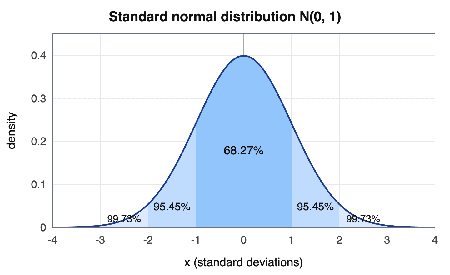
The normal distribution, or Gaussian, is the most commonly used distribution over real numbers. It is parameterized by a mean $\mu$, which is also the location of its peak, and a standard deviation $\sigma$; when the density must be evaluated many times, it is often parameterized by the precision $\beta = 1/\sigma^2$ instead [1]. Goodfellow and colleagues give two reasons why it is a sensible default when nothing else is known. First, the central limit theorem shows that the sum of many independent random variables is approximately normal, so many complicated systems can be modeled as Gaussian noise. Second, among all distributions with the same variance, the normal distribution carries the most uncertainty, so it adds the least prior knowledge to a model [1].
The multivariate normal distribution generalizes this to vectors, with a mean vector $\boldsymbol{\mu}$ and a positive definite covariance matrix $\boldsymbol{\Sigma}$. In practice the covariance is often restricted to a diagonal matrix, or to a scalar times the identity (an isotropic Gaussian), which is cheaper to evaluate [1].
Mixtures and latent variables
Richer distributions can be built by mixing simple ones. A mixture distribution first draws a component identity $c$ from a categorical distribution and then draws $x$ from that component, so $P(x) = \sum_i P(c = i) P(x \mid c = i)$ [1]. The component identity is an example of a latent variable, a random variable that is never observed directly. In a Gaussian mixture model each component is a Gaussian with its own mean and covariance, and such a model is a universal approximator of densities: with enough components it can approximate any smooth density to any nonzero error [1]. The empirical distribution of a real-valued dataset is itself a mixture, with one Dirac delta component at each training example; it is also the distribution that maximizes the likelihood of the training data [1].
Measuring how distributions differ
Information theory supplies most of the tools used to compare distributions. The self-information of an outcome is $-\log P(x)$, and the Shannon entropy $H(P) = -\mathbb{E}_{x \sim P}[\log P(x)]$ is the expected information of a draw; nearly deterministic distributions have low entropy and near-uniform ones high entropy [1].
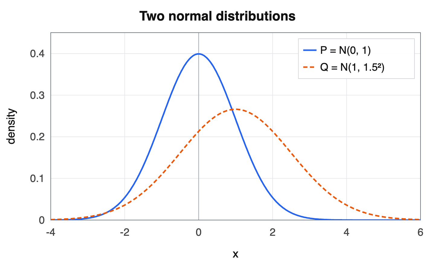
The Kullback-Leibler divergence between two distributions over the same variable is
It is non-negative and is zero only when the two distributions are equal (almost everywhere, for continuous variables), but it is not symmetric, so it is not a true distance [1]. The direction matters in practice. When a single Gaussian $q$ is fitted to a two-peaked distribution $p$, minimizing $D_{\mathrm{KL}}(p ,|, q)$ tends to spread $q$ over both peaks, while minimizing $D_{\mathrm{KL}}(q ,|, p)$ tends to lock onto one peak if the peaks are well separated [1].
The cross-entropy $H(P, Q) = -\mathbb{E}{x \sim P}[\log Q(x)]$ equals $H(P) + D{\mathrm{KL}}(P ,|, Q)$. Because $H(P)$ does not depend on $Q$, minimizing cross-entropy with respect to $Q$ is the same as minimizing the KL divergence [1].
Two other measures are prominent in generative modeling. The Jensen-Shannon divergence compares each distribution with their average mixture; it is symmetric and always defined [9]. The Earth-Mover or Wasserstein-1 distance is the smallest expected distance needed to move probability mass from one distribution to the other, taken over all joint distributions whose marginals are the two distributions being compared [9]. It is the basis of the Wasserstein loss.
Probability distributions in machine learning
The data-generating distribution
Statistical learning theory treats datasets as samples from a probability distribution. Under the usual i.i.d. assumptions, examples are independent of one another and the training and test sets are drawn from the same distribution, called the data-generating distribution $p_{\text{data}}$; this is what makes it possible to relate training error to test error [4]. The article on independently and identically distributed data covers the assumption itself, and distribution shift covers what happens when deployment data stop following the training distribution.
Maximum likelihood and loss functions
Maximum likelihood estimation chooses parameters $\theta$ of a model distribution $p_{\text{model}}(x; \theta)$ that maximize $\sum_i \log p_{\text{model}}(x^{(i)}; \theta)$ over the training examples. Dividing by the number of examples turns this into an expectation under the empirical distribution $\hat{p}{\text{data}}$, and maximizing it is equivalent to minimizing $D{\mathrm{KL}}(\hat{p}{\text{data}} ,|, p{\text{model}})$, or equivalently the cross-entropy between the empirical and model distributions [4]. Goodfellow and colleagues argue that calling only the Bernoulli or softmax negative log-likelihood "cross-entropy" is a misnomer, since any negative log-likelihood is a cross-entropy between the empirical distribution and the model [4].
This view explains why common loss functions look the way they do. Most modern neural networks are trained by maximum likelihood, so the cost is the negative log-likelihood $-\mathbb{E}\log p_{\text{model}}(y \mid x)$ [5]. The choice of output distribution then fixes the loss:
| Output distribution | Output unit | Resulting loss |
|---|---|---|
| Gaussian with fixed variance, $\mathcal{N}(y; f(x;\theta), I)$ | Linear | Mean squared error, up to scale and a constant [5] |
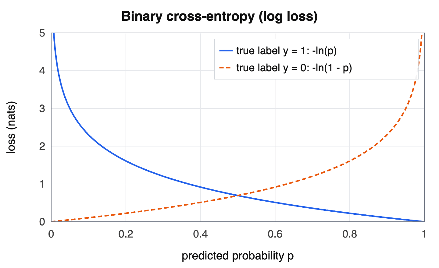
| Bernoulli over a binary label | Sigmoid | Bernoulli negative log-likelihood (binary cross-entropy, log loss) [5] |
| Categorical over $n$ classes | Softmax | Categorical cross-entropy [5] |
| Gaussian mixture | Softmax weights, means, variances | Mixture negative log-likelihood [5] |
The softmax turns a vector of logits $z$ into a categorical distribution, $p(k \mid x) = \exp(z_k) / \sum_i \exp(z_i)$ [10]. Networks with Gaussian mixture outputs, often called mixture density networks (Jacobs et al., 1991; Bishop, 1994), are used when the target can have several peaks for the same input; their mixing weights usually come from a softmax so that they form a valid categorical distribution [5]. Practitioners also reshape target and output distributions on purpose:
- Label smoothing. Szegedy and colleagues replaced the one-hot target with $q'(k) = (1 - \epsilon)\delta_{k,y} + \epsilon/K$, a mixture of the true label and a uniform distribution, to stop the model from becoming overconfident. With $K = 1000$ ImageNet classes and $\epsilon = 0.1$ they reported an improvement of about 0.2 percentage points in both top-1 and top-5 error [10]. See label smoothing.
- Temperature. Dividing logits by a temperature $T$ before the softmax produces a softer distribution when $T > 1$. Knowledge distillation as described by Hinton, Vinyals and Dean trains a small model on these soft targets at a high temperature and uses $T = 1$ after training [11].
Language models
A statistical language model learns a probability distribution over sequences of words; Bengio and colleagues described this as learning "the joint probability function of sequences of words in a language" in their 2003 neural probabilistic language model [12]. Modern language models apply the chain rule and compute the probability of a text as the product of next-token conditionals, $P(x_{1:T}) = \prod_i P(x_i \mid x_1, \ldots, x_{i-1})$ [13]. Each step of generation is therefore a draw from, or a search over, a categorical distribution over the vocabulary.
Holtzman and colleagues found that decoding for maximum probability, as in beam search, produces bland and repetitive text even from strong models, and proposed nucleus (top-p) sampling, which samples from the smallest set of tokens whose cumulative probability reaches $p$, after renormalizing [13]. Top-k sampling instead keeps a fixed number $k$ of the most probable tokens. Sampling temperature rescales the logits before the softmax; values below 1 skew the distribution toward high-probability tokens and reduce the mass in the tail [13].
Generative models
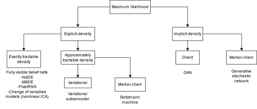
Many deep generative models are defined by how they represent a distribution over data:
- Variational autoencoders. Kingma and Welling's example model uses a standard isotropic Gaussian prior $\mathcal{N}(z; 0, I)$ over latent variables, a Gaussian (for real-valued data) or Bernoulli (for binary data) decoder, and a diagonal Gaussian approximate posterior, trained by maximizing a reparameterized variational lower bound [14]. See reparameterization trick.
- Generative adversarial networks. A generator learns to capture the data distribution while a discriminator estimates whether a sample came from the data or the generator. Goodfellow and colleagues showed that, with an optimal discriminator, the generator's objective equals $-\log 4 + 2,\mathrm{JSD}(p_{\text{data}} ,|, p_g)$, minimized only when the generator's distribution equals the data distribution [15]. The Wasserstein GAN uses the Earth-Mover distance instead; its authors reported more stable training and fewer problems such as mode collapse [9].
- Normalizing flows. Rezende and Mohamed described a normalizing flow as transforming a simple initial density into a more complex one through a sequence of invertible transformations [16]. Because the transformation is invertible, the change-of-variables formula gives the model density exactly, $p_X(x) = p_Z(f(x)) \lvert \det(\partial f(x) / \partial x^\top) \rvert$, which lets models such as Real NVP compute exact log-likelihoods and draw exact samples [17].
- Diffusion models. Sohl-Dickstein and colleagues proposed slowly destroying structure in a data distribution with an iterative forward diffusion process and learning a reverse process that restores it [18]. In denoising diffusion probabilistic models, the forward process is a Markov chain that adds Gaussian noise according to a variance schedule, and each reverse step is a Gaussian with learned parameters [19]. Song and colleagues recast this as a stochastic differential equation that carries the data distribution to a known prior, with a reverse-time equation that depends only on the score, the gradient of the log density of the noised data distribution [20]. See score matching.
Reinforcement learning
In reinforcement learning, Bellemare, Dabney and Munos argued for modeling the full distribution of returns rather than only its expectation, the value. Their categorical algorithm represents the return distribution as a discrete distribution over a fixed set of $N$ atoms between a minimum and maximum value and trains it with the cross-entropy term of a KL divergence; the 51-atom agent was evaluated on games from the Arcade Learning Environment [21].
Software
Deep learning frameworks ship distribution libraries. PyTorch's torch.distributions package, which "generally follows the design of the TensorFlow Distributions package", provides parameterizable distributions and sampling functions, including Bernoulli, Beta, Binomial, Categorical, Dirichlet, Gamma, Laplace, Multinomial, MultivariateNormal, Normal, Poisson, Uniform and MixtureSameFamily [22]. It supports the two standard ways of differentiating through random samples: the score-function estimator (REINFORCE), which needs only sample() and log_prob() and underlies policy gradient methods, and the pathwise derivative through rsample(), the reparameterization trick common in variational autoencoders [22].
Technical subtleties
A fully rigorous treatment of continuous distributions uses measure theory. Without it, paradoxes can arise: it is possible to construct two disjoint sets whose probabilities, computed naively, add up to more than 1. Measure theory characterizes which sets can be assigned probabilities consistently and gives precise meaning to statements that hold "almost everywhere", that is, except on a set of measure zero [1].
Transforming a continuous variable also changes its density in a way that is easy to get wrong. If $y = g(x)$ for an invertible, differentiable $g$, then $p_y(y) \ne p_x(g^{-1}(y))$ in general; the correct formula multiplies by $\lvert \partial x / \partial y \rvert$, and in several dimensions by the absolute determinant of the Jacobian, to account for how $g$ stretches or compresses space [1]. This correction is the same one that normalizing flows exploit [17].
Continue reading
- Cross-EntropyCross-entropy is a measure from information theory of how many bits (or nats) are needed to encode data drawn from a true probability distribution P when using a code optimized for a differentMentioned 8 times above
- Normal distributionThe normal distribution, also called the Gaussian distribution, is a continuous probability distribution defined by two parameters.Mentioned 3 times above
- KL Divergence (Kullback-Leibler Divergence)Kullback-Leibler divergence, often abbreviated KL divergence and written…Mentioned 3 times above
- Generative ModelA generative model is a class of statistical and machine learning model that learns the joint probability distribution P(X) of the observed data, or the joint distribution P(X, Y) of inputs and labelsMentioned 3 times above
- Maximum likelihood estimation (MLE)Maximum likelihood estimation (MLE) is the method of choosing the parameters of a probability model so that they make the observed data as probable as possible: given a parametric model with density (or mass)…Listed in See also
- Probabilistic Regression ModelA probabilistic regression model (also called distributional regression) is a regression model that outputs a full probability distribution over possible target values rather than a single point estimate.Listed in See also
More from See also
More to read
References
- ^1 ^2 ^3 ^4 ^5 ^6 ^7 ^8 ^9 ^10 ^11 ^12 ^13 ^14 ^15 ^16 ^17 ^18 ^19 ^20 ^21 ^22 ^23 ^24 ^25 ^26 ^27 ^28 ^29 ^30 ^31 ^32 ^33 ^34 ^35 ^36 ^37 ^38 ^39 ^40 ^41 ^42 ^43 ^44 ^45Goodfellow, Ian; Bengio, Yoshua; Courville, Aaron. "Probability and Information Theory" (Chapter 3). Deep Learning, MIT Press, 2016. deeplearningbook.org/...prob
- ^1 ^2 ^3Hájek, Alan. "Interpretations of Probability". Stanford Encyclopedia of Philosophy, first published 2002-10-21, substantive revision 2023-11-16. plato.stanford.edu/...probability-interpret
- ^1 ^2 ^3NIST/SEMATECH. "1.3.6.2. Related Distributions". e-Handbook of Statistical Methods, National Institute of Standards and Technology. itl.nist.gov/...eda362
- ^1 ^2 ^3 ^4Goodfellow, Ian; Bengio, Yoshua; Courville, Aaron. "Machine Learning Basics" (Chapter 5). Deep Learning, MIT Press, 2016. deeplearningbook.org/...ml
- ^1 ^2 ^3 ^4 ^5 ^6 ^7 ^8 ^9 ^10Goodfellow, Ian; Bengio, Yoshua; Courville, Aaron. "Deep Feedforward Networks" (Chapter 6). Deep Learning, MIT Press, 2016. deeplearningbook.org/...mlp
- ^1 ^2NIST/SEMATECH. "1.3.6.6.18. Binomial Distribution". e-Handbook of Statistical Methods, National Institute of Standards and Technology. itl.nist.gov/...eda366i
- ^1 ^2NIST/SEMATECH. "1.3.6.6.19. Poisson Distribution". e-Handbook of Statistical Methods, National Institute of Standards and Technology. itl.nist.gov/...eda366j
- ^NIST/SEMATECH. "1.3.6.6.17. Beta Distribution". e-Handbook of Statistical Methods, National Institute of Standards and Technology. itl.nist.gov/...eda366h
- ^1 ^2 ^3Arjovsky, Martin; Chintala, Soumith; Bottou, Léon. "Wasserstein GAN". arXiv:1701.07875, 2017. arxiv.org/...1701.07875
- ^1 ^2Szegedy, Christian; Vanhoucke, Vincent; Ioffe, Sergey; Shlens, Jonathon; Wojna, Zbigniew. "Rethinking the Inception Architecture for Computer Vision". arXiv:1512.00567, 2015. arxiv.org/...1512.00567
- ^Hinton, Geoffrey; Vinyals, Oriol; Dean, Jeff. "Distilling the Knowledge in a Neural Network". arXiv:1503.02531, 2015. arxiv.org/...1503.02531
- ^Bengio, Yoshua; Ducharme, Réjean; Vincent, Pascal; Jauvin, Christian. "A Neural Probabilistic Language Model". Journal of Machine Learning Research 3:1137-1155, 2003. jmlr.org/...bengio03a
- ^1 ^2 ^3Holtzman, Ari; Buys, Jan; Du, Li; Forbes, Maxwell; Choi, Yejin. "The Curious Case of Neural Text Degeneration". ICLR 2020; arXiv:1904.09751. arxiv.org/...1904.09751
- ^Kingma, Diederik P.; Welling, Max. "Auto-Encoding Variational Bayes". arXiv:1312.6114, 2013. arxiv.org/...1312.6114
- ^1 ^2Goodfellow, Ian J.; Pouget-Abadie, Jean; Mirza, Mehdi; Xu, Bing; Warde-Farley, David; Ozair, Sherjil; Courville, Aaron; Bengio, Yoshua. "Generative Adversarial Networks". arXiv:1406.2661, 2014. arxiv.org/...1406.2661
- ^Rezende, Danilo Jimenez; Mohamed, Shakir. "Variational Inference with Normalizing Flows". arXiv:1505.05770, 2015. arxiv.org/...1505.05770
- ^1 ^2Dinh, Laurent; Sohl-Dickstein, Jascha; Bengio, Samy. "Density estimation using Real NVP". ICLR 2017; arXiv:1605.08803. arxiv.org/...1605.08803
- ^1 ^2Sohl-Dickstein, Jascha; Weiss, Eric A.; Maheswaranathan, Niru; Ganguli, Surya. "Deep Unsupervised Learning using Nonequilibrium Thermodynamics". arXiv:1503.03585, 2015. arxiv.org/...1503.03585
- ^Ho, Jonathan; Jain, Ajay; Abbeel, Pieter. "Denoising Diffusion Probabilistic Models". arXiv:2006.11239, 2020. arxiv.org/...2006.11239
- ^Song, Yang; Sohl-Dickstein, Jascha; Kingma, Diederik P.; Kumar, Abhishek; Ermon, Stefano; Poole, Ben. "Score-Based Generative Modeling through Stochastic Differential Equations". arXiv:2011.13456, 2020. arxiv.org/...2011.13456
- ^Bellemare, Marc G.; Dabney, Will; Munos, Rémi. "A Distributional Perspective on Reinforcement Learning". Proceedings of the 34th International Conference on Machine Learning, 2017; arXiv:1707.06887. arxiv.org/...1707.06887
- ^1 ^2PyTorch. "Probability distributions - torch.distributions". PyTorch 2.15 documentation. docs.pytorch.org/...distributions
Improve this article
Add missing citations, update stale details, or write a clearer explanation. Anyone can edit: changes go live when you publish, and every edit is checked by an editor.
2 revisions · v2 · 4,043 words · full history
Fact-checks are independent of edits: a reviewer re-verifies the article against its sources and stamps the date. How we verify
Research and drafting on this wiki are AI-assisted, under named human editorial standards. How AI is used here
Reviewer note: Independent fact-check before publication on November 18, 2026: 78 claims checked against 22 cited and independent sources; 0 material and 2 minor corrections applied before publication.
Cite this page: AI Wiki. "Probability distribution." aiwiki.ai, updated 18 Nov 2026, fact-checked 18 Nov 2026. CC BY 4.0. https://aiwiki.ai/wiki/probability_distribution