

Jensen-Shannon divergence
The Jensen-Shannon divergence (JSD, also written JS divergence) is a measure of how different two probability distributions are. It compares each distribution with their equal-weight average: the JSD is the mean of the two Kullback-Leibler divergences from each distribution to that average mixture [2][3]. Unlike the Kullback-Leibler divergence, it is symmetric, defined for every pair of distributions, and bounded, and its square root is a metric [2][3]. Jianhua Lin's 1991 paper "Divergence measures based on the Shannon entropy" called the quantity the Jensen-Shannon divergence and worked out its main properties, including a weighted version for any finite number of distributions [1]. In machine learning it drew wide attention through the original generative adversarial network (GAN) paper [3], which showed that when the discriminator is optimal, the generator's training criterion equals $-\log 4 + 2,\mathrm{JSD}(p_{\text{data}} ,|, p_g)$ [4]. It is also used as a drift metric in model monitoring, as a consistency loss, as a distillation objective and as a layer-selection rule in large language model decoding [9][10][11][15][16].
Definition
Two distributions
For two probability distributions $P$ and $Q$ on the same space, let $M = \tfrac{1}{2}(P + Q)$ be their mixture (the pointwise average). The Jensen-Shannon divergence is
where $D_{\mathrm{KL}}$ is the Kullback-Leibler divergence [3][7]. For densities $p$ and $q$ this can be written as a single integral, $\mathrm{JSD}(p ,|, q) = \tfrac{1}{2}\int \left( p \log \frac{2p}{p+q} + q \log \frac{2q}{p+q} \right) d\mu$ [3]. Because each distribution is compared with the mixture rather than with the other distribution, Frank Nielsen describes the JSD as the total divergence to the average distribution [3].
The same quantity can be written with the entropy $H$ of information theory:
In this form it is the entropy of the mixture minus the average entropy of the parts [2][3]. Since Shannon entropy is concave, Jensen's inequality makes this difference non-negative, and the name reflects that origin: Lin derived the measure from Jensen's inequality and the Shannon entropy [1].
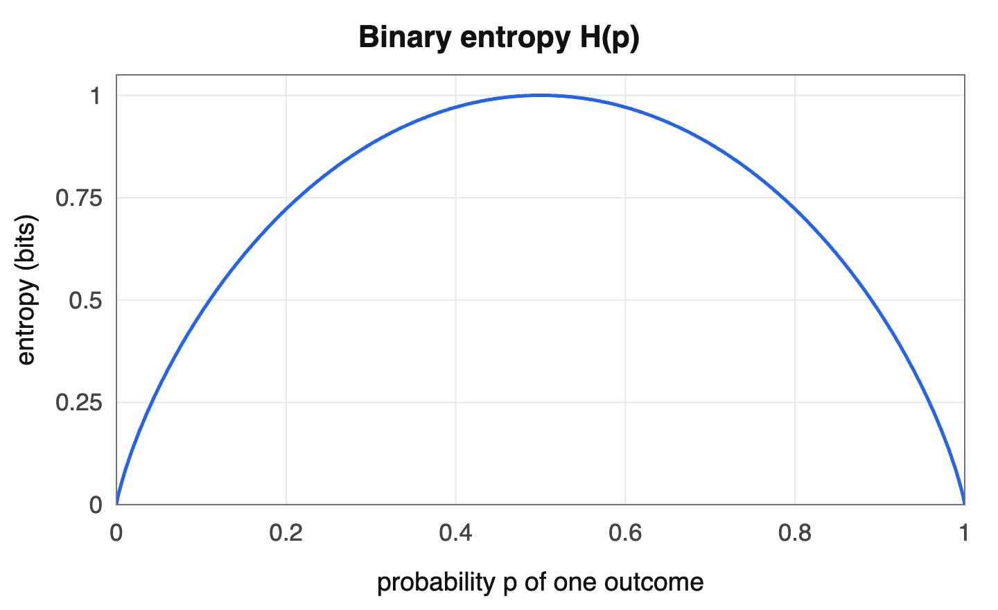
The units depend on the base of the logarithm. Lin used base 2 throughout, which gives values in bits [1]. With natural logarithms the values are in nats, and the upper bound becomes $\log 2 \approx 0.69$ [3][6].
Weighted and multi-distribution form
Lin also defined a weighted version. With weights $\pi_1, \pi_2 \ge 0$ that sum to 1, the divergence is $\mathrm{JS}_\pi(p_1, p_2) = H(\pi_1 p_1 + \pi_2 p_2) - \pi_1 H(p_1) - \pi_2 H(p_2)$, and the definition extends to $n$ distributions $p_1, \dots, p_n$ with weights $\pi_1, \dots, \pi_n$ [1]:
Lin pointed out that the ability to give each distribution its own weight suits decision problems, where the weights can be the prior probabilities of the classes [1]. Jop Briët and Peter Harremoës show that the general form equals the weighted sum of Kullback-Leibler divergences from each $p_i$ to the weighted mixture, $\sum_i \pi_i D_{\mathrm{KL}}(p_i ,|, \bar{p})$ with $\bar{p} = \sum_i \pi_i p_i$, and that this second expression can be used when the entropies are infinite [2].
Worked example
Take $P = (0.5, 0.5)$, a fair coin, and $Q = (1, 0)$, a coin that always lands heads. The Kullback-Leibler divergence $D_{\mathrm{KL}}(P ,|, Q)$ is infinite, because $Q$ gives zero probability to an outcome that $P$ allows; Lin identified this requirement (absolute continuity) as a problem with Kullback-Leibler-based measures [1]. The JSD is still finite. The mixture is $M = (0.75, 0.25)$, and computing the definition above gives:
| Quantity | Value (bits) | Value (nats) |
|---|---|---|
| $D_{\mathrm{KL}}(P ,|, M)$ | 0.2075 | 0.1438 |
| $D_{\mathrm{KL}}(Q ,|, M)$ | 0.4150 | 0.2877 |
| $\mathrm{JSD}(P ,|, Q)$ | 0.3113 | 0.2158 |
| $\sqrt{\mathrm{JSD}(P ,|, Q)}$ (JS distance) | 0.5579 | 0.4645 |
If $P = (1, 0)$ and $Q = (0, 1)$ instead, the two distributions have no outcome in common and the JSD reaches its maximum, 1 bit ($\log 2$ nats).
History and naming
Briët and Harremoës trace the general form back to R. G. Gallager, who proved in 1968 that it is a convex function of the distributions for fixed weights [2]. R. Sibson's 1969 paper "Information radius" showed applications in biology and cluster analysis, and A. K. C. Wong and M. You used the two-distribution case as a distance between random graphs [2]. Lin's paper notes that Wong and You called it the "increment of the Shannon entropy" and had conjectured, from computer simulation, that it cannot exceed 1; Lin's bounds proved the conjecture [1]. Lin also related the generalized form to the "Jensen difference" that C. R. Rao had proposed in a different context [1].
Lin's 1991 paper built the measure in steps. It first defined a directed divergence $K(p_1, p_2)$, which is the Kullback-Leibler divergence from $p_1$ to the mixture, and a symmetric sum $L(p_1, p_2) = K(p_1, p_2) + K(p_2, p_1) = 2H!\left(\tfrac{p_1+p_2}{2}\right) - H(p_1) - H(p_2)$ [1]. The weighted generalization of $L$ is what Lin termed the Jensen-Shannon divergence [1]. With equal weights, Lin's $L$ is twice the JSD as usually defined today, so formulas in the literature can differ by a factor of 2 depending on which convention an author follows; the Wasserstein GAN paper, for instance, writes the JS divergence as the plain sum of the two Kullback-Leibler terms [1][6].
The square root of the JSD is called the Jensen-Shannon distance, for example in SciPy [14]. Briët and Harremoës call it the transmission metric, after the interpretation of the JSD as the transmission rate of a communication channel [2].
Properties
| Property | Statement | Source |
|---|---|---|
| Symmetry | $\mathrm{JSD}(P ,|, Q) = \mathrm{JSD}(Q ,|, P)$ | [2][13] |
| Non-negativity | $\mathrm{JSD} \ge 0$, with equality only when $P = Q$ | [1][4] |
| Always defined | No absolute-continuity condition between $P$ and $Q$ is needed | [1][6] |
| Bounded | $0 \le \mathrm{JSD} \le \log 2$ (1 bit in base 2) | [1][3] |
| Metric | $\sqrt{\mathrm{JSD}}$ satisfies the triangle inequality | [2][3] |
| Hilbert embedding | The metric space can be isometrically embedded in a real Hilbert space | [2] |
| f-divergence | The JSD belongs to Csiszár's family of f-divergences | [1][7] |
| Convexity | The general form is convex in $(p_1, \dots, p_k)$ for fixed weights | [2] |
| Topology | Convergence in JSD is equivalent to convergence in total variation | [2][6] |
Boundedness
The upper bound follows from the definition: each term $D_{\mathrm{KL}}(P ,|, M)$ is at most $\log 2$, because $M$ is never less than half of $P$ [3]. The bound is attained when the two distributions do not overlap. Martin Arjovsky and Leon Bottou show that if two distributions lie on low-dimensional manifolds that do not perfectly align, the JSD equals $\log 2$ while both Kullback-Leibler divergences are infinite, and that this holds even when the manifolds are arbitrarily close to each other [5]. For the general weighted form, Lin showed that $\mathrm{JS}_\pi \le H(\pi)$, the entropy of the weights, which is at most 1 bit for two distributions [1].
Relation to other divergences
Lin proved that his symmetric $L$ divergence (twice the JSD, in bits) is never larger than the variational distance $V(p_1, p_2) = \sum_x |p_1(x) - p_2(x)|$. No such general upper bound in terms of the variational distance exists for the Kullback-Leibler divergence or its symmetrized form [1]. He also noted that his directed $K$ divergence coincides with the f-divergence for $f(x) = x \log \frac{2x}{1+x}$, so results about f-divergences carry over [1]. Sebastian Nowozin, Botond Cseke and Ryota Tomioka list the JSD with its generator function among the f-divergences in their f-GAN paper [7].
In terms of the topology it induces, Arjovsky, Soumith Chintala and Bottou proved that, for distributions on a compact space, a sequence converges in JSD exactly when it converges in total variation; convergence in Kullback-Leibler divergence implies it, and it implies convergence in distribution (equivalently, convergence in Wasserstein distance on a compact space) [6]. Briët and Harremoës reach the same characterization: the topology of the JS distance is that of convergence in total variation [2].
Metric property
The JSD itself is not a metric, but its square root is. Briët and Harremoës credit D. M. Endres and J. E. Schindelin with proving in 2003 that the JSD is the square of a metric [2]. Nielsen also cites Bent Fuglede and Flemming Topsøe's work on Hilbert space embedding and Igor Vajda's 2009 paper on metric divergences for this property [3]. Briët and Harremoës extended the result to a family of "Jensen divergences of order $\alpha$" built from entropies of order $\alpha$: for $\alpha \in (0, 2]$ the square root is a metric and the space embeds isometrically in a real separable Hilbert space, while for $\alpha \in (2, 3)$ it cannot be the square of a metric [2]. Briët and Harremoës point out that the metric property means results such as Banach's fixed point theorem hold for the space of probability distributions with this metric [2].
Information-theoretic interpretations
The JSD has several equivalent readings:
- Mutual information. Suppose a label $C$ is drawn with probabilities $\pi$, and then an observation $X$ is drawn from the distribution $p_C$. Lin's derivation shows that the conditional entropy $H(C \mid X)$ equals $H(\pi) - \mathrm{JS}_\pi(p_1, p_2)$, so the JSD is the mutual information between the observation and the label [1]. Briët and Harremoës state the same fact in channel language: for a discrete memoryless channel with input distribution $\pi$, the general JSD of the output distributions is the transmission rate [2]. The AugMix authors put it informally: the JSD measures the average information a sample reveals about which distribution it came from [10].
- Classification error. Because of this link to $H(C \mid X)$, the JSD bounds the Bayes probability of misclassification. Lin proved that for two classes with priors $\pi$, the Bayes error $P_e$ satisfies $\tfrac{1}{4}\left(H(\pi) - \mathrm{JS}\pi\right)^2 \le P_e \le \tfrac{1}{2}\left(H(\pi) - \mathrm{JS}\pi\right)$, and extended the bounds to $n$ classes; he noted that no similar upper bound exists in terms of the Kullback-Leibler divergence [1].
- Compression redundancy. In a coding setting where a sender switches between several source distributions and the receiver must use one code without knowing which source is active, the minimum average extra code length (the redundancy) is the general JSD, achieved by coding for the mixture [2].
- Statistical physics and statistics. Ivo Grosse and colleagues presented interpretations of the JSD in statistical physics, information theory and mathematical statistics, and derived approximations of its mean, variance and distribution for random, uncorrelated symbol sequences [12].
Role in generative adversarial networks
The original GAN objective
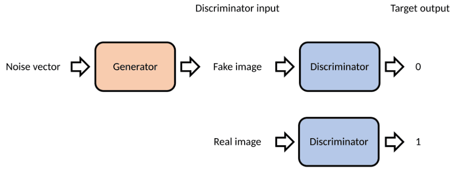
In the 2014 GAN paper by Ian Goodfellow and colleagues, a generator $G$ and a discriminator $D$ play a two-player minimax game with value function [4]
For a fixed generator, the optimal discriminator is $D^*G(x) = \frac{p{\text{data}}(x)}{p_{\text{data}}(x) + p_g(x)}$, where $p_g$ is the generator's distribution [4]. Substituting it back gives the generator's criterion
The paper identifies this expression as the Jensen-Shannon divergence between the model's distribution and the data-generating process [4]. Because the JSD is non-negative and zero only when the distributions are equal, the global minimum $-\log 4$ is reached only when $p_g = p_{\text{data}}$, meaning the generator reproduces the data distribution [4]. Arjovsky and Bottou summarize the result as: minimizing the GAN objective with respect to the generator's parameters minimizes the JSD when the discriminator is optimal [5].
The equivalence holds only in that idealized case. The GAN paper itself does not train the discriminator to optimality at each step: it alternates $k$ steps of optimizing $D$ with one step of optimizing $G$, because optimizing $D$ to completion in the inner loop is computationally prohibitive and would overfit on finite data [4]. It also recommends, as a practical change, training $G$ to maximize $\log D(G(z))$ instead of minimizing $\log(1 - D(G(z)))$, since the original term saturates early in training when $D$ can easily reject generated samples; this alternative has the same fixed point but gives stronger gradients [4].
Training problems linked to the JSD
Arjovsky and Bottou's 2017 analysis traced several GAN training problems to properties of the JSD [5]:
- Saturation at $\log 2$. They argued that both the data distribution and the generator's distribution are concentrated on low-dimensional manifolds. When those manifolds do not align, a perfect discriminator exists and the JSD is at its maximum, $\log 2$, so the divergence gives no indication of how close the generator is [5].
- Vanishing gradients. With the original $\log(1 - D(G(z)))$ cost, they proved that as the discriminator gets better the gradient on the generator goes to zero [5].
- Instability of the alternative cost. For the $-\log D$ alternative, they proved that with an optimal discriminator the generator's gradient equals the gradient of $\mathrm{KL}(P_g ,|, P_r) - 2,\mathrm{JSD}(P_g ,|, P_r)$. The JSD enters with a negative sign, which pushes the distributions apart, and the remaining reverse Kullback-Leibler term puts a high cost on unrealistic samples and a low cost on dropping modes, which they offer as an explanation for the mode dropping seen in practice [5].
As a remedy, they proposed adding noise to both real and generated samples, so that the generator's gradient becomes proportional to the gradient of the JSD between the two noisy distributions; annealing the noise then brings the original distributions together as well [5]. The follow-up Wasserstein GAN paper by Arjovsky, Chintala and Bottou replaced the JSD with the Earth-Mover (Wasserstein-1) distance [6]. Its motivating example uses a distribution on a vertical line segment through the origin and a copy shifted horizontally by $\theta$: the Wasserstein distance is $|\theta|$, while the JSD is $\log 2$ for every $\theta \ne 0$ and 0 at $\theta = 0$, so as a loss it is not continuous in $\theta$ and gives no usable gradient [6]. In experiments, the authors plotted the discriminator-based estimate of the JSD during standard GAN training and reported that it correlated poorly with sample quality and often stayed close to $\log 2 \approx 0.69$, its maximum value [6]. See Wasserstein loss and earth mover's distance for that line of work.
f-GAN and the skewed Jensen-Shannon divergence
Nowozin, Cseke and Tomioka generalized adversarial training to the whole family of f-divergences. In their framing the original GAN objective is $D_{\text{GAN}} = 2 D_{\text{JS}} - \log 4$, and the JSD is one choice among several (Kullback-Leibler, reverse Kullback-Leibler, Pearson $\chi^2$, squared Hellinger and others) that can be minimized with a variational discriminator [7].
Ferenc Huszár proposed a generalized, skewed Jensen-Shannon divergence with a parameter $0 < \pi < 1$ [8]:
It is not symmetric for $\pi \ne \tfrac{1}{2}$, but it satisfies $\mathrm{JS}\pi[P ,|, Q] = \mathrm{JS}{1-\pi}[Q ,|, P]$ [8]. Huszár showed that as $\pi \to 0$, $\mathrm{JS}_\pi / \pi$ approaches $\mathrm{KL}[P ,|, Q]$, the objective of maximum likelihood, and as $\pi \to 1$ the divergence behaves like $\mathrm{KL}[Q ,|, P]$, which favors conservative, mode-seeking models; the standard JSD sits at the midpoint [8]. He argued that adversarial training can approximately minimize this divergence, with $\pi$ set by the balance of data and model samples presented to the discriminator, and offered it as a theoretical explanation for why adversarial training tends to produce samples of higher perceived quality than maximum likelihood [8].
Other uses in machine learning
| Application | How the JSD is used | Source |
|---|---|---|
| Training-serving skew and drift | TensorFlow Data Validation accepts a jensen_shannon_divergence threshold in a feature's skew comparator; its documentation notes that this detects skew for both numeric and categorical features, while the L-infinity norm only covers categorical ones | [15] |
| Model monitoring | Google Cloud's Model Monitoring documentation lists JSD as a supported metric for input-feature and output drift on numerical features, and alongside L-infinity distance for categorical features | [16] |
| Robustness training | AugMix adds a consistency loss: the JSD among a classifier's predicted distributions for an image and two augmented versions of it, which is bounded by the logarithm of the number of classes | [10] |
| Knowledge distillation | Generalized Knowledge Distillation (GKD) for language models uses a generalized $\mathrm{JSD}(\beta)$ between teacher and student token distributions, described as bounded even for distributions with disjoint supports and interpolating between forward and reverse KL | [11] |
| LLM decoding | DoLa selects, at each decoding step, the earlier ("premature") layer whose next-token distribution has the largest JSD from the final layer's, then contrasts the two | [9] |
AugMix, from Dan Hendrycks and colleagues, computes the three-way divergence by forming the mixture $M = (p_{\text{orig}} + p_{\text{augmix1}} + p_{\text{augmix2}})/3$ and averaging the three Kullback-Leibler divergences to it; the authors report that using only the original image and one augmented copy did not perform as well [10]. This is an application of the multi-distribution form described above, used to make a neural network's outputs consistent across data augmentations.
In GKD, Rishabh Agarwal and colleagues compared forward KL, reverse KL and three settings of $\mathrm{JSD}(\beta)$ (0.1, 0.5 and 0.9) as the knowledge distillation divergence for T5 student models; in the summary comparison in their first figure, GKD used $\mathrm{JSD}(0.1)$ on the WMT translation task and forward KL on the other tasks [11]. Their $\mathrm{JSD}(\beta)$ has the same form as Huszár's skewed divergence, and they cite his result on its limiting behavior [11].
In DoLa (Decoding by Contrasting Layers), Yung-Sung Chuang and colleagues computed the JSD between the output distributions of early layers and the final layer of the 32-layer LLaMA-7B model. They found that for tokens such as named entities and dates the JSD stayed high into the upper layers, while for function words it became very small from the middle layers onward, and they used the JSD to pick which layer to contrast with [9]. DoLa is covered with related methods in contrastive decoding.
Uses outside machine learning
- Genomics and symbolic sequences. Grosse and colleagues described the JSD as widely applied to the analysis of symbolic sequences and presented a JSD-based method that segments a nonstationary sequence into stationary parts, which they applied to DNA sequences [12].
- Biology, taxonomy and clustering. Lin cited taxonomy in biology and genetics as a setting that needs a single measure of difference among more than two distributions, which the generalized JSD provides [1]. Sibson's earlier work applied the measure in biology and cluster analysis [2].
- Time series and graphs. Briët and Harremoës list its use by Rosso and colleagues to separate deterministic from stochastic behavior in a time series, and by Wong and You as a distance between random graphs [2].
- Quantum information. The quantum Jensen-Shannon divergence replaces Shannon entropy with the von Neumann entropy $S(\rho) = -\mathrm{Tr}, \rho \ln \rho$ of density matrices [2]. A. P. Majtey, P. W. Lamberti and D. P. Prato proposed it in 2005 as a measure of distinguishability between mixed quantum states and an alternative to quantum relative entropy, motivated by the classical JSD being symmetric, always well defined and bounded; they showed that it shares most of the physically relevant properties of relative entropy [13]. Briët and Harremoës relate its general form to Holevo's bound on the classical capacity of a quantum channel and proved the metric property for qubits and for pure states [2].
Variants and generalizations
| Variant | Idea | Source |
|---|---|---|
| Weighted JSD $\mathrm{JS}_\pi$ | Unequal weights on the distributions, for example class priors | [1] |
| Multi-distribution JSD | Entropy of the weighted mixture minus the weighted entropies, for any finite number of distributions | [1] |
| Skewed (generalized) JSD | $\mathrm{JS}_\pi$ that interpolates between forward and reverse KL | [8][11] |
| Jensen divergence of order $\alpha$ | Shannon entropy replaced by entropy of order $\alpha$; square root a metric for $\alpha \in (0, 2]$ | [2] |
| Quantum JSD | Von Neumann entropy of density matrices | [2][13] |
| M-JSD (abstract means) | The arithmetic mixture replaced by another mean, such as a geometric mean | [3] |
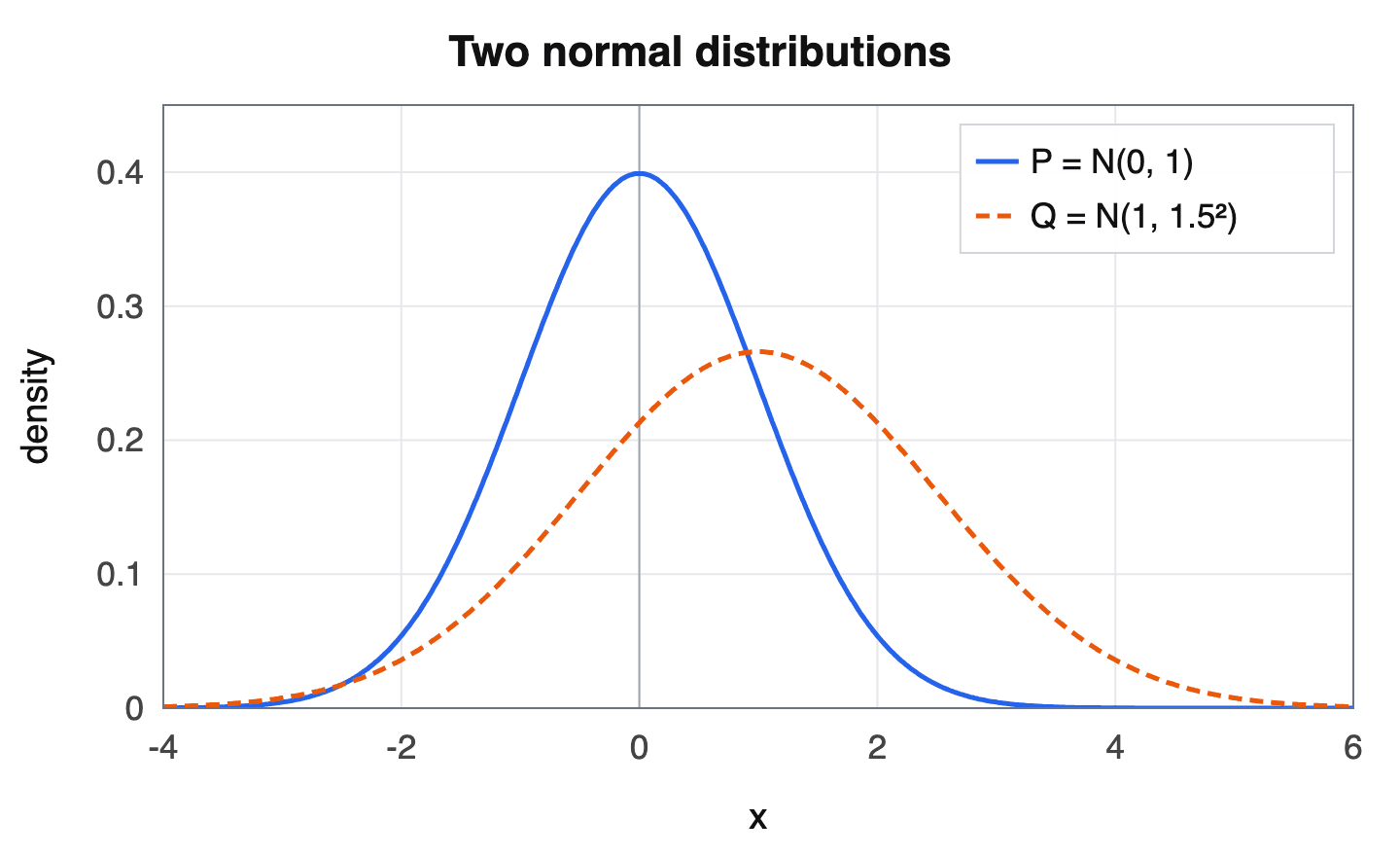
Nielsen's generalization addresses a practical limitation: the JSD between two Gaussian distributions has no closed-form expression, because a mixture of two Gaussians is not Gaussian [3]. Replacing the arithmetic mixture with a mean suited to the distribution family gives closed forms, for example a geometric-mean JSD for densities in the same exponential family (including multivariate Gaussians) and a harmonic-mean version for scale Cauchy distributions [3].
Computing the JSD
For discrete distributions the JSD is computed directly from the definition. Outcomes with zero probability under one distribution cause no difficulty, because the mixture is positive wherever either distribution is; Lin notes that his directed divergence is well defined whatever the values of the two distributions [1]. Software libraries differ in whether they return the divergence or its square root. SciPy's scipy.spatial.distance.jensenshannon, added in version 1.2.0, returns the Jensen-Shannon distance, the square root of the divergence, and normalizes its inputs if they do not sum to 1; a base argument sets the logarithm base [14]. Squaring its output gives the divergence. Because conventions also differ on the factor of $\tfrac{1}{2}$ (Lin's $L$ divergence omits it) and on the logarithm base, values reported by different papers or tools are comparable only when these choices match [1][14].
For continuous distributions known only through samples, the JSD generally has to be estimated. The GAN discriminator gives one such estimate: Arjovsky, Chintala and Bottou note that the discriminator's objective is a lower bound of $2,\mathrm{JS}(P_r, P_\theta) - 2\log 2$, so $\tfrac{1}{2} L(D, g_\theta) + \log 2$ is a lower bound on the JSD [6].
Continue reading
- EntropyEntropy is a quantitative measure of the uncertainty, randomness, or average information content in a probability distribution: for a discrete random variable it is, to within one questionMentioned 17 times above
- KL Divergence (Kullback-Leibler Divergence)Kullback-Leibler divergence, often abbreviated KL divergence and written…Mentioned 4 times above
- Wasserstein LossWasserstein loss is a loss function for training generative models that measures the distance between two probability distributions as the Wasserstein-1 distanceMentioned 3 times above
- Probability distributionA probability distribution is a description of how likely a random variable, or a set of random variables, is to take on each of its possible values.Mentioned 3 times above
- Generative adversarial networkGenerative adversarial networks (GANs) are a family of generative models trained through competition between two learned functions.Mentioned twice above
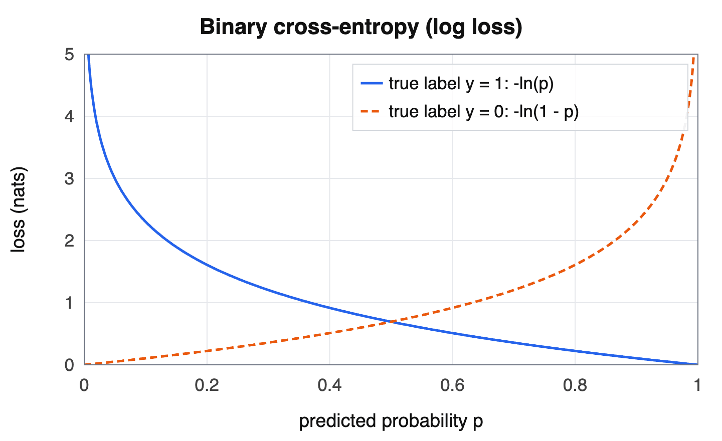
- Cross-EntropyCross-entropy is a measure from information theory of how many bits (or nats) are needed to encode data drawn from a true probability distribution P when using a code optimized for a differentListed in See also
More from See also
More to read
References
- ^1 ^2 ^3 ^4 ^5 ^6 ^7 ^8 ^9 ^10 ^11 ^12 ^13 ^14 ^15 ^16 ^17 ^18 ^19 ^20 ^21 ^22 ^23 ^24 ^25Lin, J. "Divergence measures based on the Shannon entropy". IEEE Transactions on Information Theory, vol. 37, no. 1, pp. 145-151, January 1991. doi.org/...18.61115
- ^1 ^2 ^3 ^4 ^5 ^6 ^7 ^8 ^9 ^10 ^11 ^12 ^13 ^14 ^15 ^16 ^17 ^18 ^19 ^20 ^21 ^22 ^23 ^24Briët, J.; Harremoës, P. "Properties of classical and quantum Jensen-Shannon divergence". Physical Review A, vol. 79, 052311, 2009 (arXiv:0806.4472). arxiv.org/...0806.4472
- ^1 ^2 ^3 ^4 ^5 ^6 ^7 ^8 ^9 ^10 ^11 ^12 ^13 ^14 ^15Nielsen, F. "On a generalization of the Jensen-Shannon divergence and the JS-symmetrization of distances relying on abstract means". arXiv:1904.04017, 2019 (journal version: "On the Jensen-Shannon Symmetrization of Distances Relying on Abstract Means", Entropy, vol. 21, no. 5, 485, 2019). arxiv.org/...1904.04017
- ^1 ^2 ^3 ^4 ^5 ^6 ^7 ^8Goodfellow, I. J.; Pouget-Abadie, J.; Mirza, M.; Xu, B.; Warde-Farley, D.; Ozair, S.; Courville, A.; Bengio, Y. "Generative Adversarial Networks". arXiv:1406.2661, June 2014. arxiv.org/...1406.2661
- ^1 ^2 ^3 ^4 ^5 ^6 ^7Arjovsky, M.; Bottou, L. "Towards Principled Methods for Training Generative Adversarial Networks". arXiv:1701.04862, January 2017. arxiv.org/...1701.04862
- ^1 ^2 ^3 ^4 ^5 ^6 ^7 ^8 ^9Arjovsky, M.; Chintala, S.; Bottou, L. "Wasserstein GAN". arXiv:1701.07875, 2017. arxiv.org/...1701.07875
- ^1 ^2 ^3 ^4Nowozin, S.; Cseke, B.; Tomioka, R. "f-GAN: Training Generative Neural Samplers using Variational Divergence Minimization". arXiv:1606.00709, June 2016. arxiv.org/...1606.00709
- ^1 ^2 ^3 ^4 ^5Huszár, F. "How (not) to Train your Generative Model: Scheduled Sampling, Likelihood, Adversary?". arXiv:1511.05101, November 2015. arxiv.org/...1511.05101
- ^1 ^2 ^3Chuang, Y.-S.; Xie, Y.; Luo, H.; Kim, Y.; Glass, J.; He, P. "DoLa: Decoding by Contrasting Layers Improves Factuality in Large Language Models". ICLR 2024 (arXiv:2309.03883). arxiv.org/...2309.03883
- ^1 ^2 ^3 ^4Hendrycks, D.; Mu, N.; Cubuk, E. D.; Zoph, B.; Gilmer, J.; Lakshminarayanan, B. "AugMix: A Simple Data Processing Method to Improve Robustness and Uncertainty". ICLR 2020 (arXiv:1912.02781). arxiv.org/...1912.02781
- ^1 ^2 ^3 ^4 ^5Agarwal, R.; Vieillard, N.; Zhou, Y.; Stanczyk, P.; Ramos, S.; Geist, M.; Bachem, O. "On-Policy Distillation of Language Models: Learning from Self-Generated Mistakes". ICLR 2024 (arXiv:2306.13649). arxiv.org/...2306.13649
- ^1 ^2Grosse, I.; Bernaola-Galván, P.; Carpena, P.; Román-Roldán, R.; Oliver, J.; Stanley, H. E. "Analysis of symbolic sequences using the Jensen-Shannon divergence". Physical Review E, vol. 65, 041905, 2002. doi.org/...PhysRevE.65.041905
- ^1 ^2 ^3Majtey, A. P.; Lamberti, P. W.; Prato, D. P. "Jensen-Shannon divergence as a measure of distinguishability between mixed quantum states". Physical Review A, vol. 72, 052310, 2005 (arXiv:quant-ph/0508138). arxiv.org/...0508138
- ^1 ^2 ^3SciPy developers. "scipy.spatial.distance.jensenshannon". SciPy documentation. docs.scipy.org/...y.spatial.distance.jensenshannon
- ^1 ^2TensorFlow. "Get started with TensorFlow Data Validation". TFX documentation. tensorflow.org/...get_started
- ^1 ^2Google Cloud. "Introduction to Model Monitoring". Google Cloud documentation. docs.cloud.google.com/...overview
Improve this article
Add missing citations, update stale details, or write a clearer explanation. Anyone can edit: changes go live when you publish, and every edit is checked by an editor.
1 revision · v1 · 4,048 words · full history
Fact-checks are independent of edits: a reviewer re-verifies the article against its sources and stamps the date. How we verify
Research and drafting on this wiki are AI-assisted, under named human editorial standards. How AI is used here
Reviewer note: Independent fact-check before publication on November 18, 2026: 92 claims checked against 19 cited and independent sources; 0 material and 5 minor corrections applied before publication.
Cite this page: AI Wiki. "Jensen-Shannon divergence." aiwiki.ai, updated 18 Nov 2026, fact-checked 18 Nov 2026. CC BY 4.0. https://aiwiki.ai/wiki/jensen_shannon_divergence