

Maximum a posteriori estimation
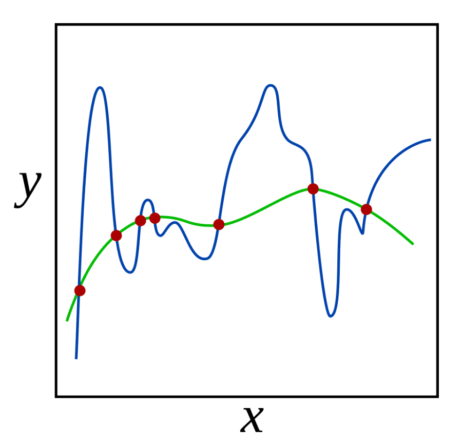
Maximum a posteriori estimation (MAP estimation) is a method of Bayesian point estimation that picks the parameter value with the highest posterior probability, or the highest posterior density when the parameter is continuous, after the observed data have been combined with a prior distribution.[1][2] It sits between maximum likelihood estimation (MLE), which ignores priors, and full Bayesian inference, which keeps the whole posterior distribution instead of reducing it to one point.[1][3] With a uniform prior the MAP estimate equals the maximum likelihood estimate.[2] In machine learning, MAP estimation gives a probabilistic interpretation of many forms of regularization: adding a penalty to a log-likelihood objective is equivalent to maximizing a posterior when the penalty equals a negative log prior. Under this reading, ridge regression and weight decay correspond to Gaussian priors and the lasso to a Laplace (double-exponential) prior.[1][2][4]
Definition
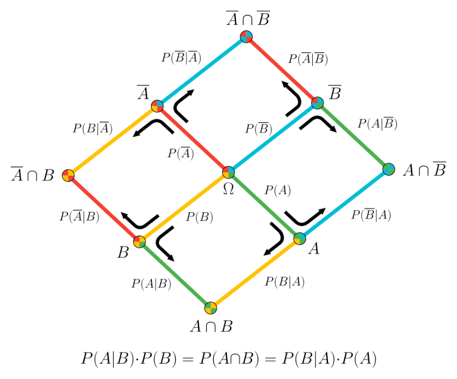
Let $\theta$ be the unknown parameters and $\mathcal{D}$ the observed data. Bayes' theorem gives the posterior $p(\theta \mid \mathcal{D}) \propto p(\mathcal{D} \mid \theta), p(\theta)$, where $p(\mathcal{D} \mid \theta)$ is the likelihood and $p(\theta)$ is the prior. The MAP estimate is the mode of this posterior:[1][2]
The normalizing constant $p(\mathcal{D})$ does not depend on $\theta$, so it can be dropped, and taking logarithms does not move the maximum. The objective therefore has two parts: the ordinary log-likelihood term used by MLE, and a log-prior term.[1][2] Equivalently, the MAP estimate minimizes the negative log-likelihood plus the negative log-prior.[2]
Bishop's textbook calls the technique "maximum posterior, or simply MAP" and introduces it as finding "the most probable value of w given the data".[3] The Goodfellow, Bengio and Courville textbook notes that for continuous parameters, the more common case, the estimate is the point of maximal probability density rather than maximal probability.[1]
Relation to maximum likelihood and full Bayesian inference
If the prior is uniform, $p(\theta) \propto 1$, the log-prior term is constant and the MAP estimate reduces to the MLE.[2] Bishop shows the same limit for Bayesian linear regression: as the Gaussian prior on the weights becomes infinitely broad, the posterior mean, which for a Gaussian posterior coincides with its mode, reduces to the maximum likelihood solution.[3] In the other direction, with no data the posterior is just the prior.[3]
MAP estimation still makes a point estimate, so Bishop notes that it "does not yet amount to a Bayesian treatment"; a fully Bayesian approach integrates over the parameters rather than fixing them at one value.[3] Murphy describes MAP estimation as an approximation to inference in the one-level model $\theta \rightarrow \mathcal{D}$, and places it in a ladder of methods that become "more Bayesian" as more of the unknowns are integrated out:[2]
| Method | What is optimized or computed |
|---|---|
| Maximum likelihood | $\hat{\theta} = \arg\max_\theta p(\mathcal{D} \mid \theta)$ |
| MAP estimation | $\hat{\theta}(\xi) = \arg\max_\theta p(\mathcal{D} \mid \theta), p(\theta \mid \xi)$ |
| ML-II (empirical Bayes) | $\hat{\xi} = \arg\max_\xi \int p(\mathcal{D} \mid \theta), p(\theta \mid \xi), d\theta$ |
| MAP-II | $\hat{\xi} = \arg\max_\xi \int p(\mathcal{D} \mid \theta), p(\theta \mid \xi), p(\xi), d\theta$ |
| Full Bayes | $p(\theta, \xi \mid \mathcal{D}) \propto p(\mathcal{D} \mid \theta), p(\theta \mid \xi), p(\xi)$ |
Here $\xi$ denotes the hyperparameters of the prior. The table follows Murphy's Probabilistic Machine Learning: An Introduction.[2]
Goodfellow, Bengio and Courville summarize the trade-off against MLE: like full Bayesian inference, MAP estimation can use information from the prior that is not present in the training data, and this reduces the variance of the estimate compared with the ML estimate, "at the price of increased bias".[1] This is an instance of the bias-variance tradeoff.
Worked examples
Coin flips with a beta prior
For a Bernoulli parameter $\theta$ (the probability of heads) with $N_1$ heads and $N_0$ tails, the MLE is $N_1 / (N_1 + N_0)$. If only one head has been observed, the MLE is $\theta = 1$, which predicts that every future toss will be heads.[2] With a $\text{Beta}(a, b)$ prior, the MAP estimate is
Choosing $a = b = 2$, a prior that weakly favors values near 0.5, gives $(N_1 + 1)/(N_1 + N_0 + 2)$. Murphy notes that this is add-one smoothing, a widely used fix for the zero-count problem.[2] With $a = b = 1$, the beta prior is uniform and the formula falls back to the MLE.[2]
Mean of a Gaussian
Murphy works through estimating the mean $\theta$ of a Gaussian with known variance $\sigma^2$ from $N$ samples with sample mean $\bar{x}$. Under a Gaussian prior $\mathcal{N}(\theta_0, \sigma^2 / \kappa_0)$, the MAP estimate is a weighted average of the sample mean and the prior mean:[2]
The estimate is biased toward $\theta_0$ whenever $w < 1$, but its variance is $w^2 \sigma^2 / N$, smaller than the $\sigma^2 / N$ of the MLE. In simulations where the prior is misspecified (prior mean 0, true mean 1), Murphy finds that moderate prior strengths ($\kappa_0 \in {1, 2}$) give lower mean squared error than the MLE, while a strong prior ($\kappa_0 = 3$) hurts. He concludes that a MAP estimate can beat the ML estimate on mean squared error as long as the prior strength is tuned appropriately.[2] Because $w = N/(N + \kappa_0)$, the weight on the data approaches 1 as the sample grows, and the prior's influence fades.
Regularization as a prior
Many penalized objectives in statistics and machine learning can be read as MAP estimation. Murphy writes the regularized objective as an average loss plus $\lambda C(\theta)$, where $\lambda$ is the regularization parameter; choosing the complexity penalty $C(\theta) = -\log p(\theta)$ with the log loss turns minimization of the objective into maximization of the log posterior, which Murphy names MAP estimation.[2] The strength of the prior then plays the role of the regularization rate.
| Penalty | Equivalent prior on each weight | Resulting method |
|---|---|---|
| Squared L2 norm, $\lambda \lVert w \rVert_2^2$ | Zero-mean Gaussian | Ridge regression, weight decay |
| L1 norm, $\lambda \lVert w \rVert_1$ | Zero-mean Laplace (double-exponential) | Lasso |
| Negative log of a Gaussian mixture density | Mixture of Gaussians with adaptive means and variances | Soft weight-sharing |
Gaussian prior: ridge regression and weight decay
For linear regression with Gaussian noise of variance $\sigma^2$ and a prior $w \sim \mathcal{N}(0, \tau^2 I)$, the MAP estimate minimizes the residual sum of squares plus $\lambda \lVert w \rVert_2^2$ with $\lambda = \sigma^2 / \tau^2$. Murphy calls this ridge regression and notes that the technique is known in general as $\ell_2$ regularization or weight decay.[2] Its closed form is $\hat{w}_{\text{MAP}} = (X^\top X + \lambda I)^{-1} X^\top y$.[2] Bishop derives the same equivalence for polynomial curve fitting, with the regularization coefficient equal to the ratio of the prior precision $\alpha$ to the noise precision $\beta$, $\lambda = \alpha / \beta$.[3] A tighter prior (smaller $\tau^2$, larger $\alpha$) means stronger regularization.
Goodfellow, Bengio and Courville give the same example for a linear regression model: a Gaussian prior $\mathcal{N}(w; 0, \tfrac{1}{\lambda} I)$ on the weights makes the log-prior term proportional to the familiar $\lambda w^\top w$ weight decay penalty, plus a constant, so "MAP Bayesian inference with a Gaussian prior on the weights thus corresponds to weight decay".[1] They conclude that many regularized estimation strategies, including maximum likelihood learning with weight decay, "can be interpreted as making the MAP approximation to Bayesian inference".[1]
Laplace prior: the lasso
In the 1996 paper that introduced the lasso, Robert Tibshirani observed that the L1 penalty is proportional to the negative log-density of the double-exponential distribution, so the lasso estimate can be derived as "the Bayes posterior mode under independent double-exponential priors" on the coefficients.[4] Comparing the double-exponential density with the normal density that is implicit in ridge regression, he noted that the former puts more mass near zero and in the tails, which matches the lasso's tendency to produce estimates that are either large or exactly zero.[4] Murphy presents the lasso as MAP estimation with a Laplace prior and calls MAP estimation with this prior $\ell_1$-regularization in general.[2] Park and Casella later built on Tibshirani's observation to develop the Bayesian lasso, a fully Bayesian treatment sampled with a Gibbs sampler that reports posterior medians and credible intervals rather than only the mode.[5]
Richer priors
Because the prior can be any density, MAP estimation gives a way to design penalties. Goodfellow, Bengio and Courville cite Nowlan and Hinton's 1992 soft weight-sharing as an example of a more complicated penalty derived from a mixture-of-Gaussians prior.[1] In that paper, the distribution of network weights is modeled as a mixture of several Gaussians whose means and variances adapt while the network trains, and a set of weights counts as simple if it has high density under the mixture.[6]
Where the correspondence stops
The equivalence is a statement about a specific objective, not about every regularizer. Goodfellow, Bengio and Courville point out that the MAP view applies only when the extra term corresponds to $\log p(\theta)$: some penalties are not the logarithm of any probability distribution, and others depend on the data, which a prior is not allowed to do.[1]
Optimizer details can also break the link between a penalty and a prior. Loshchilov and Hutter showed that L2 regularization and weight decay are equivalent for standard stochastic gradient descent when the decay is rescaled by the learning rate, but not for adaptive gradient methods such as Adam. They proposed decoupling the weight decay step from the gradient update, a variant they named AdamW, and published the work at ICLR 2019.[7]
Computing the MAP estimate
MAP estimation is an optimization problem, so the tools used for MLE usually carry over with an extra term in the objective. With a conjugate prior the estimate often has a closed form, as in the beta-Bernoulli and ridge examples above.[2] In latent-variable models the expectation-maximization (EM) algorithm can be adapted: for a Gaussian mixture model, Murphy shows that the E step is unchanged and only the M step is modified to include the log prior, for example with a Dirichlet prior on the mixture weights.[2]
The prior can also remove degenerate solutions that make maximum likelihood fail:
- Collapsing variances in mixture models. The likelihood of a Gaussian mixture can be driven to infinity by centering one component on a single data point and shrinking its variance toward zero. Murphy calls this the "collapsing variance problem" and describes MAP estimation as an easy solution.[2]
- Separable data in logistic regression. When the training data are linearly separable, maximum likelihood drives the weights to infinite magnitude and gives no way to prefer one separating hyperplane over another. Bishop notes that this singularity can be avoided by including a prior and finding a MAP solution, or equivalently by adding a regularization term.[3]
- Zero counts. As in the coin-flip example, a prior keeps a probability estimate away from exactly 0 or 1 when an outcome has not yet been observed.[2]
Decision-theoretic view
In Bayesian decision theory a point estimate is chosen to minimize the posterior expected loss. For a discrete quantity such as a class label under the zero-one loss, the expected loss of a guess is one minus its posterior probability, so the optimal guess is the most probable label, which Murphy identifies as the mode of the posterior, the MAP estimate.[2] Other losses lead to other estimators; for example, the conditional mean is the Bayes estimator under squared error.[8]
For continuous parameters the link is less direct. Bassett and Deride note that it is "commonly accepted" that MAP estimators are a limiting case of Bayes estimators with zero-one loss, give a counterexample showing the claim is false in general, and supply a level-set condition on posterior densities under which it holds.[9] In Bayesian inverse problems, Burger and Lucka describe a frequent matter of debate over whether the MAP estimate or the conditional mean should be preferred, in which MAP has been "classically discredited" for being only asymptotically a Bayes estimator. They construct convex Bayes cost functions based on Bregman distances for which the MAP estimate is the exact Bayes estimator in linear inverse problems with log-concave priors.[8]
Most probable configurations of latent variables
The same "take the most probable value" idea is applied to hidden variables in probabilistic graphical models. Bishop distinguishes two tasks: maximizing each variable's marginal separately, and finding the configuration that jointly has the largest probability. The max-sum algorithm solves the second task exactly on tree-structured graphs.[3] In a hidden Markov model this algorithm is the Viterbi algorithm, used for example to find the most probable phoneme sequence for a series of acoustic observations. Bishop warns that the sequence of individually most probable states can differ from the most probable sequence and can even have zero probability.[3]
Two well-known applications use the MAP name directly:
| Year | Work | Use of MAP estimation |
|---|---|---|
| 1984 | Stuart Geman and Donald Geman, image restoration | A stochastic relaxation algorithm with gradual "annealing" computes the MAP estimate of an original image from a degraded one, using a Gibbs distribution (Markov random field) image model.[10] |
| 1994 | Jean-Luc Gauvain and Chin-Hui Lee, speech recognition | A framework for MAP estimation of hidden Markov models with Gaussian mixture observation densities, using Dirichlet and normal-Wishart priors, applied to parameter smoothing and model adaptation.[11] |
The Geman and Geman paper's "annealing theorem" gives a temperature schedule, in the manner of simulated annealing, that guarantees convergence to the global maxima of the posterior distribution; the authors note that in practice the schedule may be too slow and used it only as a guide.[10] Gauvain and Lee extended the forward-backward and segmental k-means training algorithms with MAP formulas and argued that Bayesian learning could serve as a unified approach for a range of speech recognition applications.[11]
MAP as a starting point for approximate Bayesian inference
A MAP estimate is often the first step of a fuller Bayesian analysis. The Laplace approximation fits a Gaussian centered on the MAP estimate, with covariance given by the inverse of the Hessian of the negative log posterior at that point. Bishop uses it for Bayesian logistic regression,[3] and Murphy notes that it is easy to apply because existing optimizers find the MAP estimate, although it can approximate a skewed posterior poorly.[2]
In deep learning, Daxberger and colleagues observe that ordinary training of a neural network with a loss and a regularizer already yields a MAP estimate, because the loss terms can be identified with log-likelihoods and the regularizer with a log-prior. Their 2021 NeurIPS paper, "Laplace Redux", argues that a Laplace approximation can then be added after training, even to a downloaded network, to turn a point-estimate model into a Bayesian neural network. It also released a PyTorch library, laplace, for the purpose.[12]
Limitations and criticism
- No uncertainty. A MAP estimate is a single point. Murphy notes that the posterior mode "can be a poor summary of the posterior" for that reason, and that the posterior mean is more robust because it integrates over the whole parameter space.[2] Quantities such as credible intervals and predictive distributions require the posterior itself, or an approximation to it.[3]
- Dependence on parameterization. A probability density changes under a nonlinear change of variables by a Jacobian factor, so, as Bishop puts it, the location of the maximum of a density depends on the choice of variable.[3] The MAP estimate of a transformed parameter is therefore not in general the transform of the MAP estimate. Druilhet and Marin write that MAP estimators and highest posterior density sets are often criticized for paradoxical behavior caused by this lack of equivariance under reparametrization; they proposed a new version of the MAP estimator that avoids it and that coincides with the equivariant maximum likelihood estimator when the prior is non-informative.[13] Bishop contrasts a density with an ordinary function, which transforms without the Jacobian factor, and notes that the likelihood is a function of the parameter rather than a probability distribution over it.[3]
- Multiple modes. A posterior can have several local maxima, and an optimizer reports only one of them. Park and Casella give an example in which one form of Bayesian lasso prior produces a bimodal joint posterior, with one mode near the least-squares solution and another near the model with the coefficient set to zero.[5]
- Sensitivity to the prior. The MAP estimate inherits the prior's assumptions. In Murphy's Gaussian-mean example, a prior centered on the wrong value improves error only when its strength is tuned; a strong wrong prior makes the estimate worse than the MLE.[2]
Continue reading
- RegularizationRegularization is any deliberate change to a learning problem or training algorithm intended to improve performance on data that were not used to fit the model.Mentioned 10 times above
- EstimatorAn estimator is a rule, function, or algorithm that takes observed data and produces a value intended to approximate some unknown quantity, typically a parameter of a probability distribution or a function…Mentioned 9 times above
- Bayesian inferenceBayesian inference is a method of statistical inference in which Bayes' theorem is used to update the probability of a hypothesis as new evidence or data becomes available.Mentioned 6 times above
- Maximum likelihood estimation (MLE)Maximum likelihood estimation (MLE) is the method of choosing the parameters of a probability model so that they make the observed data as probable as possible: given a parametric model with density (or mass)…Listed in See also
- Prior beliefA prior belief, also called the prior distribution or simply the prior, is the probability distribution that expresses what is known or assumed about an unknown parameter before any data is observed.Listed in See also
- Variational InferenceVariational inference (VI), also called variational Bayes (VB), is a method in machine learning and statistics that approximates an intractable posterior distribution by turning Bayesian inference into an…Listed in See also
More to read
References
- ^1 ^2 ^3 ^4 ^5 ^6 ^7 ^8 ^9 ^10 ^11Goodfellow, Ian; Bengio, Yoshua; Courville, Aaron. "Deep Learning", Chapter 5 "Machine Learning Basics", Section 5.6.1 "Maximum A Posteriori (MAP) Estimation", pp. 136-137. MIT Press, 2016. deeplearningbook.org/...ml
- ^1 ^2 ^3 ^4 ^5 ^6 ^7 ^8 ^9 ^10 ^11 ^12 ^13 ^14 ^15 ^16 ^17 ^18 ^19 ^20 ^21 ^22 ^23 ^24 ^25 ^26Murphy, Kevin P. "Probabilistic Machine Learning: An Introduction", Sections 4.5 (Regularization and MAP estimation), 4.6.2.6-4.6.2.7, 4.6.5.3 (Empirical priors), 4.6.8.2 (Laplace approximation), 4.7.6.4, 5.1.2.1, 8.7.3.4, 11.3 and 11.4. MIT Press, 2022 (online version of 18 April 2025). probml.github.io/...book1
- ^1 ^2 ^3 ^4 ^5 ^6 ^7 ^8 ^9 ^10 ^11 ^12 ^13Bishop, Christopher M. "Pattern Recognition and Machine Learning", Sections 1.2.1 (p. 18), 1.2.3 (p. 22), 1.2.5-1.2.6 (p. 30), 3.3.1 (p. 153), 4.3.2 (p. 206), 4.5.1 (p. 218, Laplace approximation), 8.4.5 (pp. 411-415) and 13.2.5 (p. 629). Springer, 2006. microsoft.com/...ion-and-Machine-Learning-2006.pdf
- ^1 ^2 ^3Tibshirani, Robert. "Regression Shrinkage and Selection via the Lasso". Journal of the Royal Statistical Society, Series B (Methodological), 58(1), pp. 267-288, 1996. jstor.org/...2346178
- ^1 ^2Park, Trevor; Casella, George. "The Bayesian Lasso". Journal of the American Statistical Association, 103(482), pp. 681-686, June 2008. doi.org/...016214508000000337
- ^Nowlan, Steven J.; Hinton, Geoffrey E. "Simplifying Neural Networks by Soft Weight-Sharing". Neural Computation, 4(4), pp. 473-493, July 1992. doi.org/...neco.1992.4.4.473
- ^Loshchilov, Ilya; Hutter, Frank. "Decoupled Weight Decay Regularization". International Conference on Learning Representations (ICLR), 2019. arXiv:1711.05101. arxiv.org/...1711.05101
- ^1 ^2Burger, Martin; Lucka, Felix. "Maximum a posteriori estimates in linear inverse problems with log-concave priors are proper Bayes estimators". Inverse Problems, 30(11), 114004, 2014. doi.org/...114004
- ^Bassett, Robert; Deride, Julio. "Maximum a posteriori estimators as a limit of Bayes estimators". Mathematical Programming, 174, pp. 129-144, 2019 (published online January 2018). arXiv:1611.05917. arxiv.org/...1611.05917
- ^1 ^2Geman, Stuart; Geman, Donald. "Stochastic Relaxation, Gibbs Distributions, and the Bayesian Restoration of Images". IEEE Transactions on Pattern Analysis and Machine Intelligence, PAMI-6(6), pp. 721-741, November 1984. doi.org/...TPAMI.1984.4767596
- ^1 ^2Gauvain, Jean-Luc; Lee, Chin-Hui. "Maximum a posteriori estimation for multivariate Gaussian mixture observations of Markov chains". IEEE Transactions on Speech and Audio Processing, 2(2), pp. 291-298, April 1994. doi.org/...89.279278
- ^Daxberger, Erik; Kristiadi, Agustinus; Immer, Alexander; Eschenhagen, Runa; Bauer, Matthias; Hennig, Philipp. "Laplace Redux: Effortless Bayesian Deep Learning". Advances in Neural Information Processing Systems (NeurIPS), 2021. arXiv:2106.14806. arxiv.org/...2106.14806
- ^Druilhet, Pierre; Marin, Jean-Michel. "Invariant HPD credible sets and MAP estimators". Bayesian Analysis, 2(4), pp. 681-691, 2007. doi.org/...07-BA227
Improve this article
Add missing citations, update stale details, or write a clearer explanation. Anyone can edit: changes go live when you publish, and every edit is checked by an editor.
2 revisions · v2 · 3,228 words · full history
Fact-checks are independent of edits: a reviewer re-verifies the article against its sources and stamps the date. How we verify
Research and drafting on this wiki are AI-assisted, under named human editorial standards. How AI is used here
Reviewer note: Independent fact-check before publication on November 18, 2026: 68 claims checked against 16 cited and independent sources; 0 material and 6 minor corrections applied before publication.
Cite this page: AI Wiki. "Maximum a posteriori estimation." aiwiki.ai, updated 18 Nov 2026, fact-checked 18 Nov 2026. CC BY 4.0. https://aiwiki.ai/wiki/maximum_a_posteriori