

Receptive field
A receptive field is the part of a sensory space in which a stimulus can change the activity of a given neuron, or, in an artificial neural network, the region of the input that can affect the value of a given unit [1][14]. The term began in physiology: C. S. Sherrington used it in 1906 for the area of the body surface where a stimulus could trigger a reflex, and H. K. Hartline applied it in 1938 to the patch of retina whose illumination drives a single optic nerve fiber [1]. David Hubel and Torsten Wiesel's studies of receptive fields in the cat visual cortex, recognized with a share of the 1981 Nobel Prize in Physiology or Medicine, described a hierarchy of simple and complex cells [6][7]. Kunihiko Fukushima took that hierarchy as the model for his 1980 neocognitron, whose cells share connection patterns across positions and whose receptive fields grow with depth [8].
In a convolutional neural network, the receptive field of a unit in a convolutional layer is set by the kernel sizes, strides and dilations of the layers beneath it, and it can be computed exactly [11]. A 2016 study by Wenjie Luo, Yujia Li, Raquel Urtasun and Richard Zemel showed that the input pixels inside that region do not contribute equally: their influence falls off roughly like a Gaussian from the center, so the effective receptive field is only a fraction of the theoretical one [14]. Later designs, from deformable convolutions to large-kernel CNNs and visual state space models, have used the effective receptive field to motivate or evaluate their choices [15][16][19].
Origin of the term
Sherrington's 1906 book The Integrative Action of the Nervous System used "receptive field" for a region of skin from which a reflex could be elicited [1]. Hartline carried the idea over to single sensory neurons in his 1938 recordings from optic nerve fibers, writing that responses could be obtained in a given fiber "only upon illumination of a certain restricted region of the retina, termed the receptive field of the fiber" [1][2]. From there the term spread to other neurons of the visual pathway and to the other senses [1].
Jose-Manuel Alonso and Yao Chen, in a review for Scholarpedia, give a definition meant to cover all modalities: the receptive field is the portion of sensory space that can elicit neuronal responses when stimulated [1]. That space can have one dimension (for example the carbon chain length of an odorant), two (a patch of skin) or several (position, time and stimulus features for a visual neuron), and the response can be counted as spikes or can include subthreshold changes in membrane potential [1].
Receptive fields in the visual system
Center-surround organization
In 1953 Stephen Kuffler described two classes of retinal ganglion cells, which he called "on-center" and "off-center" [3][6]. The receptive field of each consists of two concentric, mutually antagonistic regions, a center and a surround, one excitatory and one inhibitory [6]. An on-center cell responds to a light spot on a dark background and an off-center cell to a dark spot on a light background, and the term center-surround organization dates to Kuffler's paper [1]. Because center and surround oppose each other, these cells respond less to diffuse light than to a spot that just fills the center; Hubel later pointed out that this lets a cell's response change little when overall illumination drops, for example when the sun goes behind a cloud [6]. Most neurons of the retina and the visual thalamus have small receptive fields of this concentric type, and their profiles can be modeled closely with a difference of Gaussians [1].
Hubel and Wiesel: simple and complex cells
After a meeting with Kuffler and Wiesel in the spring of 1958, Hubel joined Wiesel in Kuffler's laboratory at the Wilmer Institute of Ophthalmology at Johns Hopkins Hospital; their plan was to extend Kuffler's approach from the retina to the brain by mapping receptive fields with small spots of light [6]. At first the cortical cells would not respond to their spots and rings of light [6]. In Hubel's account of their first real discovery, during an unusually stable recording from one cell that lasted nine hours, the cell suddenly fired vigorously when the edge of a glass slide being inserted into the ophthalmoscope cast a faint straight shadow on the retina, and it did so only for a narrow range of line orientations [6]. They published their first paper on receptive fields of single neurons in the cat's striate cortex in The Journal of Physiology in 1959, followed in 1962 by a longer paper on receptive fields, binocular interaction and functional architecture in the cat's visual cortex [4][5].
The 1962 paper gave the first classification of cortical cells by receptive field structure [1]. Hubel and Wiesel defined simple cells by four criteria [1]:
- the receptive field can be divided into distinct excitatory and inhibitory regions;
- there is summation within each excitatory or inhibitory part;
- the excitatory and inhibitory regions are antagonistic;
- responses to stationary or moving spots of different shapes can be predicted from a map of those regions.
Unlike retinal and geniculate fields, the subregions of a simple cell are separated by parallel straight lines, so the cell prefers a slit, dark bar or edge at one orientation, and moving the line sideways off the boundary sharply reduces the response [6]. In complex cells, an optimally oriented line works anywhere in the receptive field. Hubel and Wiesel proposed that a complex cell pools inputs from many simple cells with the same preferred orientation but slightly different positions [6]. They also described cells, perhaps 10 to 20 percent of those in area 17 of the cat or monkey, that respond best to a line of limited length and less when it is extended, a property they called end stopping [6].
The Nobel Assembly at the Karolinska Institutet awarded half of the 1981 Nobel Prize in Physiology or Medicine jointly to Hubel and Wiesel "for their discoveries concerning 'information processing in the visual system'" (the other half went to Roger Sperry) [7]. The press release described a step-wise analysis of the retinal image by cells arranged in columns, each cell responsible for a specific detail of the pattern [7].
Size, eccentricity and context
Visual receptive fields range from a few minutes of arc to tens of degrees [1]. Size increases at each successive stage of the visual pathway, and within a stage it increases with eccentricity, the distance from the point of fixation; retinal ganglion cells in the fovea have the smallest fields, which is one reason peripheral vision is coarse [1]. In primates, neurons in primary visual cortex (V1) near the fovea have fields of about 0.5 to 2 degrees, while neurons in inferotemporal cortex have fields of around 30 degrees and respond selectively to objects and faces more than to exact position [1].
Modern studies add a time dimension. A spatiotemporal receptive field plots the spatial field at different delays between stimulus and response, and different response timing across subregions helps explain direction-selective neurons [1]. Receptive fields in V1 are also not fixed: measured size can be more than twice as large with low-contrast stimuli as with high-contrast ones, and responses to a faint line can be enhanced by high-contrast collinear lines placed outside the receptive field [1]. Receptive fields of cortical neurons that get direct thalamic input can be modeled with Gabor functions, the product of a sinusoid and a Gaussian [1].
Receptive fields in other senses
| Modality | What defines the receptive field | Notes |
|---|---|---|
| Somatosensory | A region of the body surface; stimuli include touch, vibration, temperature or pain | Fields are smallest at the fingertips and largest on the thigh and calf; the two-point discrimination threshold is under 5 mm at the fingertips and about 40 mm at the thigh [1] |
| Auditory (spectrotemporal) | The range of sound frequencies that drive a neuron, over time | The cochlea maps low tones at its apex and high tones at its base [1] |
| Auditory (spatial) | A region of auditory space | Built by circuits comparing intensity and timing between the two ears; some midbrain neurons show center-surround organization [1] |
| Olfactory | Odor dimensions such as molecular carbon chain length | Much less studied; early olfactory cells often have inhibitory surrounds [1] |
Receptive fields in artificial neural networks
From the neocognitron to convolutional networks
Fukushima's neocognitron, published in Biological Cybernetics in 1980, drew an explicit correspondence between its layers and the Hubel and Wiesel hierarchy model [8]. Fukushima summarized that hierarchy as one in which a cell at a higher stage responds to a more complicated feature, has a larger receptive field, and is less sensitive to shifts in stimulus position [8]. In his network, all S-cells in one cell-plane share the same pattern of input connections, shifted from cell to cell, so they have receptive fields of the same function at different positions; deeper layers have larger receptive fields, and in the last module each C-cell's receptive field covers the whole input layer [8]. A modern convolutional layer keeps both ideas: each neuron connects only to a local region of the previous layer, and the same weights are shared across positions [9].
Two uses of the term
In deep learning, "receptive field" is used in two related senses. Stanford's CS231n course notes use it for the spatial extent of a neuron's connections to the previous layer, which is the same as the filter size of a convolutional filter [9]. Analyses of deep networks, such as those by Luo and colleagues and by Araujo and colleagues, more often use it for the region of the original input that can affect a unit several layers up; Luo and colleagues note that, unlike a unit in a fully connected layer, a convolutional unit depends only on such a region, and anything outside it has no effect on the unit's value [11][14].
"Effective receptive field" is also ambiguous. The VGG paper by Karen Simonyan and Andrew Zisserman says a stack of two 3x3 convolutional layers "has an effective receptive field of 5 × 5" and three such layers a 7x7 one, meaning the full input region covered [10]. Luo and colleagues later used the same phrase for the smaller, center-weighted part of that region whose pixels have a non-negligible effect on the output [14].
Computing the theoretical receptive field
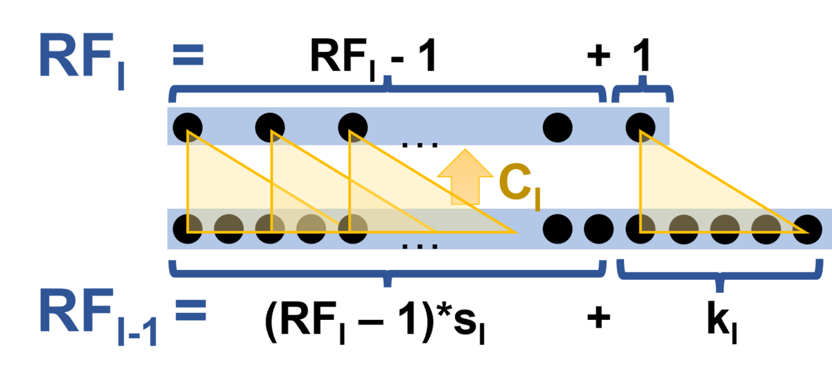
André Araujo, Wade Norris and Jack Sim gave closed-form expressions for receptive fields in a 2019 Distill article [11]. For a single-path network of $L$ layers, where layer $l$ has kernel size $k_l$ and stride $s_l$, the receptive field size $r_0$ of one output feature, measured in input pixels along one axis, is
which follows from the backward recurrence $r_{l-1} = s_l \cdot r_l + (k_l - s_l)$ starting at $r_L = 1$ [11]. Padding does not affect the size, only where the region lies [11]. The article also gives the start and end coordinates of the region and the spacing between the centers of neighboring features' receptive fields, which equals the product of all strides (the effective stride) [11]. A dilated layer with dilation factor $\alpha$ is handled by replacing $k$ with $\alpha(k-1)+1$ [11]. For networks with several paths, such as those with residual or inception branches, the receptive field of an aligned network is the largest receptive field among the paths; in a misaligned network it may not be shift-invariant [11].
Two consequences follow from the formula. In a network without striding, each extra layer adds $k-1$ pixels, so depth grows the receptive field linearly, whereas a stride or pooling step multiplies the contribution of every later layer [11][14]. Using the formula, Araujo and colleagues computed the receptive fields of the final feature maps of several TF-Slim image classifiers [11]:
| Model (TF-Slim name) | Receptive field (pixels) | Effective stride | Effective padding |
|---|---|---|---|
| AlexNet (alexnet_v2) | 195 | 32 | 64 |
| VGG-16 (vgg_16) | 212 | 32 | 90 |
| MobileNet v1 (mobilenet_v1) | 315 | 32 | 126 |
| ResNet-50 (resnet_v1_50) | 483 | 32 | 239 |
| Inception v2 (inception_v2) | 699 | 32 | 318 |
| ResNet-101 (resnet_v1_101) | 1027 | 32 | 511 |
| Inception v3 (inception_v3) | 1311 | 32 | 618 |
| ResNet-152 (resnet_v1_152) | 1507 | 32 | 751 |
| Inception v4 (inception_v4) | 2071 | 32 | 998 |
| Inception-ResNet v2 (inception_resnet_v2) | 3039 | 32 | 1482 |
The authors observed that receptive fields grew as architectures deepened and that in recent networks they usually cover the whole input image [11]. Plotting ImageNet top-1 accuracy against receptive field size for these models, they saw a roughly logarithmic relationship, and they framed a large receptive field as a likely necessary but by no means sufficient condition for high accuracy, alongside depth, width, residual connections and batch normalization [11]. They noted, for example, that VGG-16 needs about 27 times the FLOPs of MobileNet yet has a smaller receptive field [11].
Ways to enlarge the receptive field
- Stacking small kernels. VGG used 3x3 filters throughout, "the smallest size to capture the notion of left/right, up/down, center"; three stacked 3x3 layers cover the same 7x7 region as one 7x7 layer while adding two more nonlinearities and using fewer parameters [10]. In the same paper, a shallower network in which each pair of 3x3 layers was replaced by one 5x5 layer (same receptive field) had a top-1 error 7 percent higher on a center crop [10].
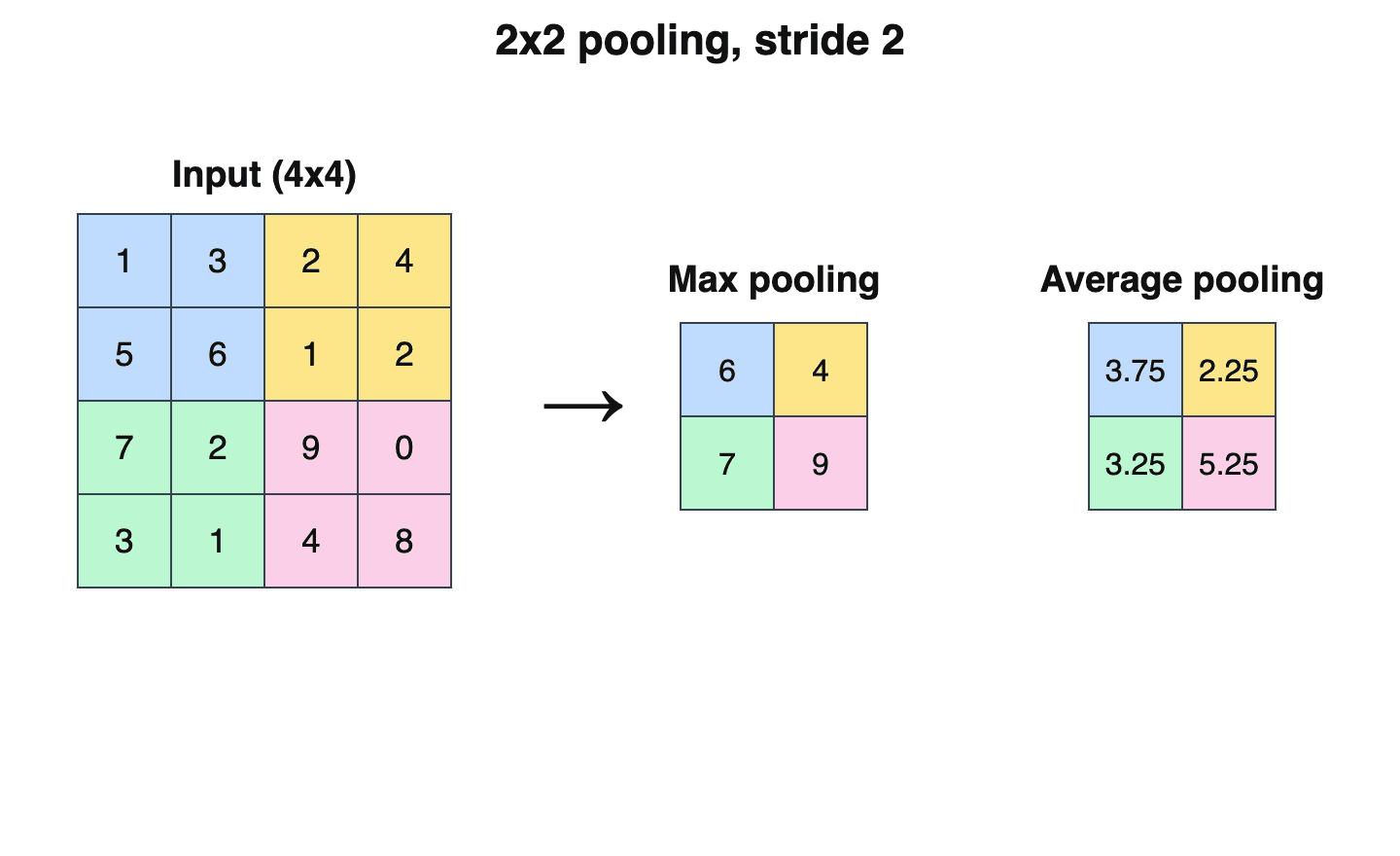
- Strides and pooling. Downsampling increases the receptive field multiplicatively rather than linearly [14].
- Dilated convolutions. Fisher Yu and Vladlen Koltun's ICLR 2016 paper on multi-scale context aggregation used 3x3 filters with dilation doubling at each layer; the receptive field then grows exponentially (3x3, 7x7, 15x15, and in general $(2^{i+2}-1) \times (2^{i+2}-1)$) while the parameter count grows only linearly, without losing resolution [12]. Their context module for semantic segmentation reached a 67x67 receptive field [12].
- Dilated causal convolutions for sequences. WaveNet applied the same idea to raw audio, repeating blocks of dilations 1, 2, 4, up to 512; each such block has a receptive field of size 1024 [13]. The authors traced some shortcomings partly to receptive field limits: generated speech lacked long-range coherence partly because the receptive field covered only about 300 milliseconds, and they suggested that occasional unnatural prosody in text-to-speech could be due to a 240 millisecond receptive field being too short for long-term pitch dependencies [13].
The effective receptive field
Luo, Li, Urtasun and Zemel, all at the University of Toronto, presented "Understanding the Effective Receptive Field in Deep Convolutional Neural Networks" at NIPS 2016 in Barcelona [14]. Their starting observation was that central pixels in a receptive field can reach the output through many more paths than pixels near its edge, so they should matter more [14].
Definition and theory
The paper measures the impact of input pixel $x^0_{i,j}$ on a central output unit $y_{0,0}$ by the partial derivative $\partial y_{0,0} / \partial x^0_{i,j}$, computed with backpropagation by setting the gradient to 1 at the chosen output and 0 elsewhere [14]. The effective receptive field (ERF) is the region of input pixels with non-negligible impact [14]. For a linear stack of $n$ convolutional layers, the authors showed that this impact is the $n$-fold convolution of the kernel with itself, which by the central limit theorem tends toward a Gaussian [14]. Taking one standard deviation as the ERF radius gives a size of order $\sqrt{n}$; for a uniform kernel of size $k$ (weights $1/k$) it is
Since the theoretical receptive field grows linearly in $n$, the ERF shrinks relative to it at a rate of $O(1/\sqrt{n})$, a result the authors called surprising [14]. The same analysis carries over to random weights through the variance of the gradients, and to ReLU networks under simplifying assumptions [14].
Main findings
| Factor | Effect reported by Luo et al. (2016) [14] |
|---|---|
| Depth | ERF size grew with a fitted log-log slope of 0.56 against layer count, and the ERF-to-theoretical ratio with a slope of -0.43, consistent with $\sqrt{n}$ growth and $1/\sqrt{n}$ shrinkage |
| Nonlinearity | Random-weight linear networks gave clean Gaussian ERFs; adding ReLU made them somewhat less Gaussian |
| Dropout | Does not change the Gaussian shape |
| Subsampling (stride 2) | Enlarges the ERF substantially |
| Dilated convolution | Enlarges the ERF substantially, with a rectangular shape |
| Skip connections | Make ERFs smaller |
| Training | ERFs start small at random initialization and grow during training |
In a CIFAR-10 experiment, a ResNet with 17 residual blocks and no downsampling had a theoretical receptive field of 74x74, larger than the 32x32 image, but its ERF did not fully fill the image [14]. In a CamVid segmentation model with a theoretical receptive field of 505x505, the ERF had a diameter of about 100 at the start of training and about 150 at the end [14]. The authors proposed an initialization that scales down weights at the center of each kernel and up at the edges; it sometimes gave a 30 percent training speed-up on CIFAR-10, but the benefit was not consistent, and they suggested architectural changes such as sparser, wider connections as a more fundamental fix [14].
Araujo and colleagues made the same point in their Distill article: pixels near the center of the receptive field have more paths to a feature and therefore carry more weight [11].
Later work
Deformable convolution
Deformable convolutional networks, proposed in 2017 by Jifeng Dai and colleagues, add learned offsets to the regular sampling grid of a convolution [15]. The authors cited the ERF result as evidence that even top-layer units may lack a large enough receptive field, and showed that stacked deformable layers adjust their receptive field to object scale and shape; on PASCAL VOC images the sampling spread of deformable filters correlated with object size [15].
Large kernels and vision transformers
The ConvNeXt paper (Zhuang Liu and colleagues, CVPR 2022) noted that non-local self-attention gives each transformer layer a global receptive field, while the convolutional standard since VGG had been to stack small kernels [17]. Testing depthwise kernels from 3x3 to 11x11, it found ImageNet top-1 accuracy rose from 79.9 percent at 3x3 to 80.6 percent at 7x7 and then saturated [17]. RepLKNet (Xiaohan Ding and colleagues, CVPR 2022) went further, using depthwise kernels as large as 31x31; its authors reported that adding layers, as in going from ResNet-101 to ResNet-152, did little to enlarge ERFs, while large kernels produced much larger ERFs and a higher shape bias, and they attributed much of the model's performance to those ERFs [16].
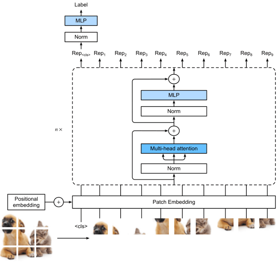
In the original Vision Transformer paper, Alexey Dosovitskiy and colleagues measured each attention head's "attention distance", the average image distance over which it integrates information, and described it as analogous to receptive field size in CNNs [18]. Some heads attended to most of the image even in the lowest layers, others stayed local, and attention distance increased with network depth [18].
State space models
ERF maps are also used to compare newer vision backbones. VMamba (Yue Liu and colleagues, NeurIPS 2024), a visual state space model based on Mamba, compared ERF maps before and after training for ResNet-50, ConvNeXt-T, Swin-T, DeiT-S, HiViT-T, Vim-S and VMamba-T [19]. Only DeiT, HiViT, Vim and VMamba showed global ERFs; the others remained local despite their theoretical potential for global coverage [19]. A paper accepted as a NeurIPS 2026 poster extended ERF analysis to Mamba sequence models, including a pretrained Mamba-370M, relating the discretized state parameters to the shape of the ERF and reporting that changing the initialization of the state matrix shifts the ERF tail as predicted [20].
Comparison with biological receptive fields
The analogy between biological and artificial receptive fields is loose. Biological receptive fields are measured by stimulating a neuron and recording its firing, they change with contrast and context, and they have a temporal structure [1]. A CNN unit's theoretical receptive field is fixed by the architecture, and its ERF is defined through gradients [11][14]. Luo and colleagues drew two connections in their discussion. In the "what" and "where" pathways of the mammalian visual system, receptive fields grow and spatial organization loosens until neurons respond to objects such as faces anywhere in the visual field; an ERF much smaller than the theoretical field suggests instead that deep CNN representations may keep position information [14]. They also suggested that, because CNN receptive fields are Gaussian, the networks may naturally form something like the fovea's high-resolution center and coarse periphery [14].
Continue reading
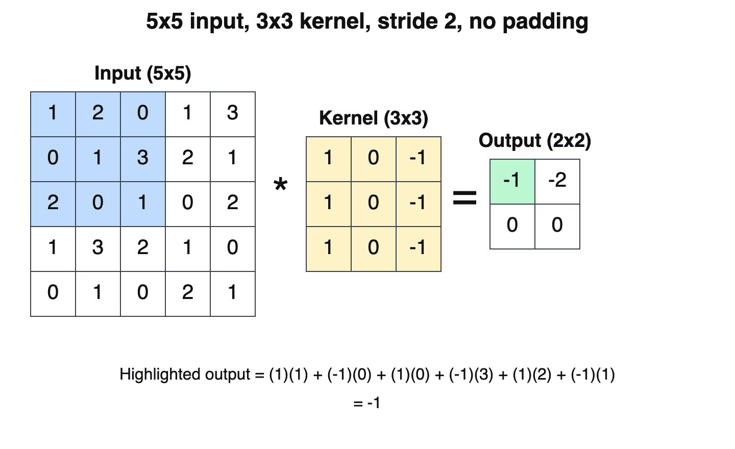
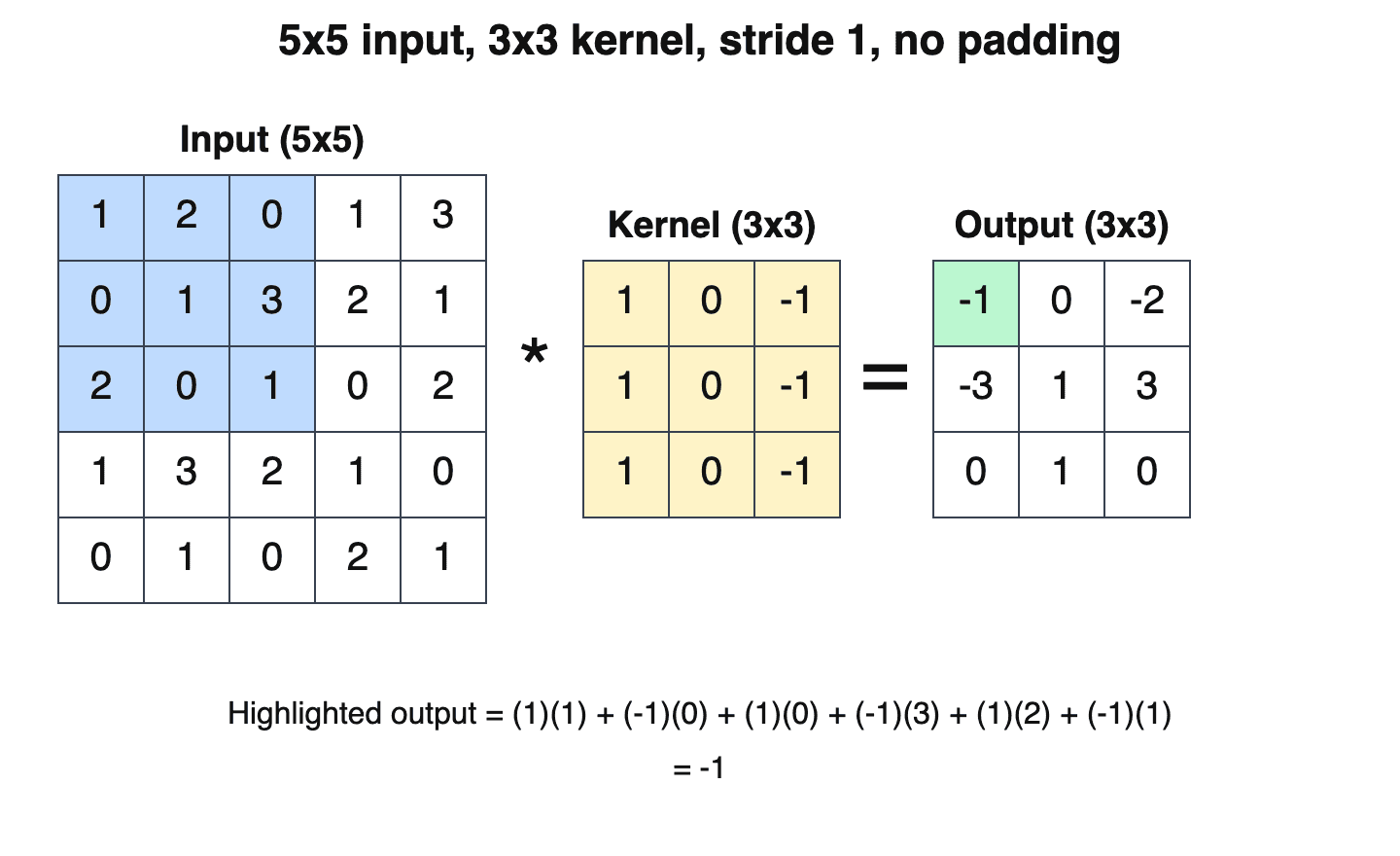
- StrideStride is the step size by which a filter (or pooling window) moves across the input in a convolutional neural network (CNN): a stride of 1 shifts the filter one position at a time and visits every location…Mentioned 9 times above
- Convolutional LayerA convolutional layer is the core building block of a convolutional neural network (CNN): it slides a small set of learnable filters (also called kernels) across the input, computing a convolution (technically…Mentioned 5 times above
- Convolutional Neural NetworkA convolutional neural network (CNN, or ConvNet) is a neural network that uses convolution-like linear operators in at least some layers.Mentioned twice above
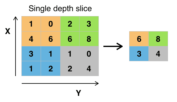
- PoolingPooling is a downsampling operation in neural networks that aggregates each local region of a feature map into a single summary valueMentioned twice above
- Vision TransformerThe Vision Transformer (ViT) is a deep learning architecture that represents an image as a sequence of fixed-size patches and processes that sequence with a Transformer encoder.Mentioned twice above
- Convolutional FilterA convolutional filter (also called a kernel or feature detector) is a small matrix of learnable weights that slides across an input and computes a dot product at each position to produce a feature map.Listed in See also
More from See also
More to read
Topics:Computer VisionDeep LearningModel ArchitectureNeural Networks
References
- ^1 ^2 ^3 ^4 ^5 ^6 ^7 ^8 ^9 ^10 ^11 ^12 ^13 ^14 ^15 ^16 ^17 ^18 ^19 ^20 ^21 ^22Alonso, Jose-Manuel; Chen, Yao. "Receptive field". Scholarpedia, 4(1):5393, 2009. doi:10.4249/scholarpedia.5393. scholarpedia.org/...Receptive_field
- ^Hartline, H. K. "The response of single optic nerve fibers of the vertebrate eye to illumination of the retina". American Journal of Physiology, 121(2):400-415, 1938. doi.org/...ajplegacy.1938.121.2.400
- ^Kuffler, Stephen W. "Discharge patterns and functional organization of mammalian retina". Journal of Neurophysiology, 16(1):37-68, 1953. doi.org/...jn.1953.16.1.37
- ^Hubel, D. H.; Wiesel, T. N. "Receptive fields of single neurones in the cat's striate cortex". The Journal of Physiology, 148(3):574-591, October 1959. doi.org/...jphysiol.1959.sp006308
- ^Hubel, D. H.; Wiesel, T. N. "Receptive fields, binocular interaction and functional architecture in the cat's visual cortex". The Journal of Physiology, 160(1):106-154, January 1962. doi.org/...jphysiol.1962.sp006837
- ^1 ^2 ^3 ^4 ^5 ^6 ^7 ^8 ^9 ^10Hubel, David H. "Evolution of ideas on the primary visual cortex, 1955-1978: a biased historical account". Nobel lecture, NobelPrize.org, 8 December 1981. nobelprize.org/...hubel-lecture.pdf
- ^1 ^2 ^3The Nobel Assembly at the Karolinska Institutet. "The Nobel Prize in Physiology or Medicine 1981 - Press release". NobelPrize.org, 9 October 1981. nobelprize.org/...press-release
- ^1 ^2 ^3 ^4Fukushima, Kunihiko. "Neocognitron: A self-organizing neural network model for a mechanism of pattern recognition unaffected by shift in position". Biological Cybernetics, 36(4):193-202, April 1980. doi.org/...BF00344251
- ^1 ^2Stanford University. "CS231n Convolutional Neural Networks for Visual Recognition: Convolutional Neural Networks". CS231n course notes. cs231n.github.io/convolutional-networks
- ^1 ^2 ^3Simonyan, Karen; Zisserman, Andrew. "Very Deep Convolutional Networks for Large-Scale Image Recognition". ICLR 2015; arXiv:1409.1556, 2014. arxiv.org/...1409.1556
- ^1 ^2 ^3 ^4 ^5 ^6 ^7 ^8 ^9 ^10 ^11 ^12 ^13 ^14 ^15Araujo, André; Norris, Wade; Sim, Jack. "Computing Receptive Fields of Convolutional Neural Networks". Distill, 4 November 2019. doi:10.23915/distill.00021. distill.pub/...computing-receptive-fields
- ^1 ^2Yu, Fisher; Koltun, Vladlen. "Multi-Scale Context Aggregation by Dilated Convolutions". ICLR 2016; arXiv:1511.07122, 2015. arxiv.org/...1511.07122
- ^1 ^2van den Oord, Aaron; Dieleman, Sander; Zen, Heiga; Simonyan, Karen; Vinyals, Oriol; Graves, Alex; Kalchbrenner, Nal; Senior, Andrew; Kavukcuoglu, Koray. "WaveNet: A Generative Model for Raw Audio". arXiv:1609.03499, 2016. arxiv.org/...1609.03499
- ^1 ^2 ^3 ^4 ^5 ^6 ^7 ^8 ^9 ^10 ^11 ^12 ^13 ^14 ^15 ^16 ^17 ^18 ^19 ^20Luo, Wenjie; Li, Yujia; Urtasun, Raquel; Zemel, Richard. "Understanding the Effective Receptive Field in Deep Convolutional Neural Networks". Advances in Neural Information Processing Systems 29 (NIPS 2016). proceedings.neurips.cc/...1288b3eb986afaa-Abstract
- ^1 ^2 ^3Dai, Jifeng; Qi, Haozhi; Xiong, Yuwen; Li, Yi; Zhang, Guodong; Hu, Han; Wei, Yichen. "Deformable Convolutional Networks". ICCV 2017; arXiv:1703.06211, 2017. arxiv.org/...1703.06211
- ^1 ^2Ding, Xiaohan; Zhang, Xiangyu; Zhou, Yizhuang; Han, Jungong; Ding, Guiguang; Sun, Jian. "Scaling Up Your Kernels to 31x31: Revisiting Large Kernel Design in CNNs". CVPR 2022; arXiv:2203.06717, 2022. arxiv.org/...2203.06717
- ^1 ^2Liu, Zhuang; Mao, Hanzi; Wu, Chao-Yuan; Feichtenhofer, Christoph; Darrell, Trevor; Xie, Saining. "A ConvNet for the 2020s". CVPR 2022; arXiv:2201.03545, 2022. arxiv.org/...2201.03545
- ^1 ^2Dosovitskiy, Alexey; et al. "An Image is Worth 16x16 Words: Transformers for Image Recognition at Scale". ICLR 2021; arXiv:2010.11929, 2020. arxiv.org/...2010.11929
- ^1 ^2 ^3Liu, Yue; Tian, Yunjie; Zhao, Yuzhong; Yu, Hongtian; Xie, Lingxi; Wang, Yaowei; Ye, Qixiang; Jiao, Jianbin; Liu, Yunfan. "VMamba: Visual State Space Model". NeurIPS 2024; arXiv:2401.10166, 2024. arxiv.org/...2401.10166
- ^Li, Zy. "Spectral Measures of Mamba Conductances Predict and Shape Effective Receptive Fields". NeurIPS 2026 poster. neurips.cc/...153177
Improve this article
Add missing citations, update stale details, or write a clearer explanation. Anyone can edit: changes go live when you publish, and every edit is checked by an editor.
2 revisions · v2 · 4,078 words · full history
Fact-checks are independent of edits: a reviewer re-verifies the article against its sources and stamps the date. How we verify
Research and drafting on this wiki are AI-assisted, under named human editorial standards. How AI is used here
Reviewer note: Independent fact-check before publication on November 18, 2026: 96 claims checked against 20 cited and independent sources; 0 material and 7 minor corrections applied before publication.
Cite this page: AI Wiki. "Receptive field." aiwiki.ai, updated 18 Nov 2026, fact-checked 18 Nov 2026. CC BY 4.0. https://aiwiki.ai/wiki/receptive_field