

SIFT (scale-invariant feature transform)
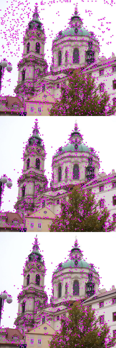
SIFT (Scale-Invariant Feature Transform) is an algorithm for detecting distinctive local points in an image and describing the patch around each one with a 128-number vector, so that the same physical point can be matched across photographs taken at different scales, rotations, viewpoints and lighting conditions. David G. Lowe of the University of British Columbia introduced it at the International Conference on Computer Vision (ICCV) in Corfu in September 1999 and gave the full treatment in a 2004 paper in the International Journal of Computer Vision (IJCV).[1][2] Lowe explained the name by saying the method "transforms image data into scale-invariant coordinates relative to local features".[2]
SIFT became the standard hand-crafted local feature of the 2000s. It was used for object recognition, robot localization and mapping, panorama stitching, large-scale 3D reconstruction from photo collections, and as the low-level descriptor in "bag of visual words" image retrieval and classification systems.[2][15][16][17][18] The University of British Columbia held a US patent on the method (US 6,711,293), which expired in March 2020; afterwards OpenCV moved SIFT into its main repository.[3][4][7] Learned features built with deep learning have since overtaken SIFT on many benchmarks,[19][22] but careful benchmarking has shown that a well-tuned SIFT pipeline remains a strong baseline, and as of November 2026 it is still the default feature extractor in the COLMAP structure-from-motion software.[24][25]
Background
Matching images through a sparse set of interest points goes back to Moravec's 1981 work on stereo matching with a corner detector, which Harris and Stephens improved in 1988 into the widely used Harris corner detector.[2] In 1997 Schmid and Mohr showed that Harris corners combined with a rotation-invariant local descriptor could recognize objects against a large image database despite clutter and occlusion.[2] Lowe's starting point was a weakness he saw in those detectors: they examine the image at a single scale, so when the size of an object changes between two images they respond to different points, and a matcher has to try descriptors at many scales.[1]
Lowe instead located keypoints in a scale space, building on Tony Lindeberg's work on scale selection and on earlier uses of the difference-of-Gaussian function by Crowley and Parker.[1][2] The 1999 paper also tied the design to biology. Lowe wrote that the features "share similar properties with neurons in inferior temporal cortex that are used for object recognition in primate vision", and the descriptor was based on a model of the behavior of complex cells in the cerebral cortex.[1] The 2004 paper explains that such neurons respond to a gradient at a particular orientation and spatial frequency while allowing its position to shift over a small receptive field, and credits an unpublished model by Edelman, Intrator and Poggio as the inspiration.[2]
Publication history
| Date | Event |
|---|---|
| 1999-03-08 | US provisional patent application filed for the method[3][4] |
| September 1999 | "Object recognition from local scale-invariant features" presented at ICCV 1999, Corfu, Greece (pp. 1150-1157)[1][3] |
| 2000-03-06 | US patent application 09/519,893 filed by the University of British Columbia[4] |
| 2004-03-23 | US Patent 6,711,293 granted[4] |
| 2004 | "Distinctive image features from scale-invariant keypoints", IJCV vol. 60, no. 2, pp. 91-110[2][3] |
| July 2005 | Version 4 of Lowe's compiled SIFT demo program released[3] |
| 2011-11-08 | The 1999 paper receives the ICCV Test-of-Time award in Barcelona[6] |
| March 2020 | Patent expires[3][4] |
| July 2020 | OpenCV 4.4.0 moves SIFT into the main OpenCV repository[7] |
The 1999 conference paper describes the first version. It builds a Gaussian image pyramid with a smoothing of $\sigma = \sqrt{2}$ and resamples between levels with a pixel spacing of 1.5, finds extrema of the difference of Gaussians, and creates a 160-element "SIFT key" from orientation planes sampled on a 4x4 grid at the detection scale plus a 2x2 grid one octave higher.[1] In that version each image produced on the order of 1,000 keys, extraction took under a second, and the full recognition system ran in under two seconds.[1]
The 2004 journal paper, dated January 5, 2004 and accepted for publication that year, reworked the detector and descriptor.[2] It added sub-pixel and sub-scale localization using a method developed by Matthew Brown (published with Lowe in 2002), rejected low-contrast and edge-like points, organized scale space into octaves, and replaced the two-scale key with the 128-element descriptor that became standard.[2] Lowe called the journal paper "the most complete and up-to-date reference" for the detector.[3] Crossref metadata lists the IJCV article in the November 2004 issue.[27]
Algorithm
The 2004 paper describes four stages, arranged as a cascade in which cheap tests run first and the more expensive operations run only on locations that pass them.[2]
Scale-space extrema detection
The scale space of an image $I(x, y)$ is the family of blurred images $L(x, y, \sigma) = G(x, y, \sigma) * I(x, y)$, where $G$ is a Gaussian kernel of standard deviation $\sigma$ and $*$ is convolution; Lowe cites Koenderink and Lindeberg for the result that, under reasonable assumptions, the Gaussian is the only possible scale-space kernel.[2] SIFT searches for extrema of the difference-of-Gaussian (DoG) function:[2]
where $k$ is a constant ratio between neighboring scales. The DoG is cheap, because the blurred images $L$ are needed anyway, and it closely approximates the scale-normalized Laplacian of Gaussian, $\sigma^2 \nabla^2 G$, which Lindeberg showed is needed for true scale invariance. From the heat diffusion equation, $G(x, y, k\sigma) - G(x, y, \sigma) \approx (k - 1)\sigma^2 \nabla^2 G$, and since $(k-1)$ is the same at every scale it does not move the extrema.[2]
Each octave (a doubling of $\sigma$) is divided into $s$ intervals, so $k = 2^{1/s}$, and $s + 3$ blurred images are produced per octave. After each octave the image is downsampled by taking every second pixel.[2] A sample point is kept as a candidate only if it is larger or smaller than all 26 of its neighbors: eight in the same DoG image and nine in each of the scales above and below. Most points fail after the first few comparisons, which keeps the search cheap.[2]
Lowe chose the sampling settings experimentally on 32 real images subjected to synthetic rotation, scaling, affine stretch, brightness and contrast change and noise. Repeatability was highest with 3 scales per octave, and a prior smoothing of $\sigma = 1.6$ gave close to optimal repeatability at reasonable cost. The input image is first doubled in size with linear interpolation, which raises the number of stable keypoints by almost a factor of four.[2] A typical 500x500-pixel image yields about 2,000 stable features, depending on image content and parameters.[2]
Keypoint localization
Each candidate is refined by fitting a 3D quadratic function to nearby samples, following Brown's method. Using the Taylor expansion of $D$ around the sample point, the offset of the true extremum is[2]
where $\mathbf{x} = (x, y, \sigma)^T$. If the offset exceeds 0.5 in any dimension, the extremum is closer to another sample and the fit is repeated there. Candidates whose interpolated value $|D(\hat{\mathbf{x}})|$ is below 0.03 (with pixel values scaled to [0, 1]) are discarded as low contrast.[2]
The DoG also responds strongly along edges, where a point is poorly localized along the edge direction. SIFT rejects such points using the 2x2 Hessian $\mathbf{H}$ of $D$ at the keypoint. Rather than computing eigenvalues, it checks the ratio of principal curvatures through the trace and determinant:[2]
with $r = 10$ in the paper. The test costs fewer than 20 floating point operations per keypoint. In the paper's 233x189-pixel example, 832 initial extrema fell to 729 after the contrast threshold and to 536 after the edge test.[2]
Orientation assignment
To make the descriptor invariant to rotation, each keypoint receives an orientation from local gradient directions. Gradient magnitudes and orientations are computed by pixel differences in the blurred image $L$ closest to the keypoint's scale and collected into a 36-bin orientation histogram covering 360 degrees, weighted by gradient magnitude and by a Gaussian window with $\sigma$ 1.5 times the keypoint scale.[2] The highest peak sets the orientation, and any other peak within 80% of it creates an additional keypoint at the same location and scale with that orientation. About 15% of points receive multiple orientations, and Lowe reported that these contribute significantly to matching stability. A parabola fitted to the three histogram values around each peak refines the angle.[2]
Keypoint descriptor
The descriptor is computed in a coordinate frame rotated to the keypoint orientation. Gradient samples from a 16x16 array around the keypoint are weighted by a Gaussian window with $\sigma$ equal to half the descriptor width and accumulated into a 4x4 grid of orientation histograms with 8 bins each, giving $4 \times 4 \times 8 = 128$ values.[2] Trilinear interpolation spreads each sample across neighboring spatial and orientation bins, so that the descriptor does not change abruptly when a gradient moves from one bin to another. Because a gradient can shift by up to 4 sample positions and still fall in the same histogram, the descriptor tolerates the small local distortions caused by 3D viewpoint change.[2]
To reduce the effect of lighting, the vector is normalized to unit length, which cancels a uniform change in contrast; a uniform change in brightness has no effect because gradients are differences of pixel values. To limit non-linear effects such as camera saturation, every element is then clipped at 0.2 and the vector is normalized again, a value Lowe set experimentally.[2] In tests with a 50-degree tilt of a planar surface and 4% image noise, matching improved as the grid grew up to 4x4 with 8 orientations; larger descriptors made results worse by becoming more sensitive to distortion.[2]
Summary of parameters
| Parameter | Value in the 2004 paper[2] |
|---|---|
| Scales sampled per octave ($s$) | 3 |
| Prior smoothing per octave | $\sigma = 1.6$ |
| Initial image upsampling | 2x (linear interpolation) |
| Contrast threshold on $\lvert D(\hat{\mathbf{x}}) \rvert$ | 0.03 |
| Edge threshold (curvature ratio $r$) | 10 |
| Orientation histogram | 36 bins, window $\sigma$ = 1.5 x keypoint scale |
| Extra orientation peaks | within 80% of the highest peak |
| Descriptor layout | 4x4 histograms x 8 orientations = 128 dimensions |
| Descriptor clipping before renormalization | 0.2 |
| Nearest-neighbor distance ratio | reject above 0.8 |
Matching and object recognition
SIFT descriptors are compared by Euclidean distance. Lowe found that a global distance threshold works poorly because some descriptors are much more discriminative than others. His alternative, often called the ratio test, compares the distance to the closest neighbor with the distance to the second-closest neighbor from a different object. Rejecting matches with a ratio above 0.8 eliminated 90% of false matches while discarding fewer than 5% of correct ones in his experiments.[2] Later benchmarks still use the ratio test as a standard matching step.[24]
Exact nearest-neighbor search in 128 dimensions is no faster than exhaustive search with structures such as the k-d tree, so Lowe used the approximate Best-Bin-First algorithm that Beis and Lowe had published in 1997. Stopping after 200 candidates gave a speedup of about two orders of magnitude over exact search on a database of 100,000 keypoints while losing less than 5% of correct matches.[2] (See approximate nearest-neighbor search.)
For object recognition, matched keypoints vote for object poses (location, scale and orientation) in a generalized Hough transform implemented with a hash table. Lowe chose this over RANSAC because correct matches can be less than 1% of the total, and he noted that methods such as RANSAC perform poorly when inliers fall much below 50%.[2] Clusters of at least 3 votes are checked by a least-squares fit of an affine transformation, outliers are removed, and a probabilistic model accepts the object if the probability of a correct interpretation exceeds 0.98.[2] On a 2 GHz Pentium 4, recognizing all the objects in the paper's example scenes took less than 0.3 seconds.[2] Lowe reported that textured planar surfaces could be recognized reliably over rotations in depth of up to 50 degrees, but 3D objects only over about 30 degrees.[2]
Evaluation and comparisons
Lowe's own tests showed orientation assignment remaining accurate 95% of the time even with ±10% pixel noise, and final matching accuracy staying above 50% out to a 50-degree viewpoint change of a planar surface.[2] He noted that the method is not fully affine invariant, and that affine-invariant detectors such as Mikolajczyk's Harris-affine keep better repeatability beyond about 50 degrees, at higher computational cost.[2]
A widely cited independent comparison was Krystian Mikolajczyk and Cordelia Schmid's "A performance evaluation of local descriptors" (IEEE TPAMI, 2005). It compared shape context, steerable filters, PCA-SIFT, differential invariants, spin images, SIFT, complex filters, moment invariants and cross-correlation, and found that the ranking was mostly independent of the region detector and that "the SIFT-based descriptors perform best".[9] The same paper introduced GLOH (gradient location and orientation histogram), a SIFT extension that it showed outperforming SIFT.[9] In their 2006 SURF paper, Herbert Bay and colleagues described SIFT as "the most appealing descriptor for practical uses, and hence also the most widely used nowadays", while noting that its high dimensionality slows matching.[11]
Patent and licensing
The method was patented in the United States as US 6,711,293, "Method and apparatus for identifying scale invariant features in an image and use of same for locating an object in an image", with Lowe as inventor and the University of British Columbia as assignee.[4] The patent claims priority from a provisional application filed on March 8, 1999, was filed on March 6, 2000, and was granted on March 23, 2004.[4] In 2011 UBC said it had licensed SIFT to more than a dozen companies.[6] Lowe's page on the detector states that the patent "expired as of March 7, 2020"; Google Patents lists it as expired, with an anticipated expiration date of 2020-03-06.[3][4]
Lowe's page offers his older 2005 demo program (version 4, July 2005) as compiled binaries for Linux and Windows, kept for historical purposes, and points to Andrea Vedaldi's VLFeat as a good publicly available implementation.[3] The patent shaped how the open-source library OpenCV shipped the algorithm:
| OpenCV release | Change |
|---|---|
| 2.3 beta (June 2011) | Added new "patent-free" BRIEF and ORB descriptors[7] |
| 2.4 beta (April 2012) | Moved SIFT and SURF to a separate nonfree module "to indicate possible legal issues of using those algorithms in user applications"[7] |
| 3.0 alpha (August 2014) | Moved SIFT, SURF and other detectors to the xfeatures2d module of the separate opencv_contrib repository[7] |
| 4.3.0 (April 2020) | Enabled SIFT in opencv_contrib by default, without the NONFREE build option, "due patents expiration"[7] |
| 4.4.0 (July 2020) | Moved SIFT into the main repository because the patent had expired[7] |
| 5.1.0 (November 2026) | Added an OpenCL implementation of the SIFT detector and descriptor for UMat input, up to 1.87x faster than the CPU version at 1080p[8] |
The release notes for OpenCV 5.0-alpha list SIFT among the detectors that remain in the renamed Features module, while several other classical detectors moved to opencv_contrib.[8]
Variants and successors
The success of SIFT produced many descriptors that modified or replaced parts of it, often to cut computation or to remove the patent restriction.
| Method | Year | Authors | Relationship to SIFT |
|---|---|---|---|
| PCA-SIFT | 2004 | Yan Ke, Rahul Sukthankar | Keeps SIFT's keypoints but applies principal component analysis to the normalized gradient patch, giving a shorter vector (20 dimensions in most of the paper's experiments)[10] |
| GLOH | 2005 | Krystian Mikolajczyk, Cordelia Schmid | Log-polar location grid with a 272-bin histogram reduced to 128 dimensions by PCA[9] |
| SURF | 2006 | Herbert Bay, Tinne Tuytelaars, Luc Van Gool | Hessian-based detector and distribution-based descriptor computed with integral images; its detector ran more than 3 times faster than DoG[11] |
| Dense SIFT in spatial pyramids | 2006 | Svetlana Lazebnik, Cordelia Schmid, Jean Ponce | SIFT descriptors of 16x16 patches computed on a regular grid with 8-pixel spacing instead of at keypoints[16] |
| ASIFT (affine SIFT) | 2009 | Jean-Michel Morel, Guoshen Yu | Simulates changes of camera axis orientation and then applies SIFT, giving full affine invariance at about twice SIFT's cost with a two-resolution scheme[14] |
| ORB | 2011 | Ethan Rublee, Vincent Rabaud, Kurt Konolige, Gary Bradski | Rotation-invariant, noise-resistant binary descriptor based on BRIEF, reported to be two orders of magnitude faster than SIFT while performing comparably in many situations[12] |
| RootSIFT | 2012 | Relja Arandjelović, Andrew Zisserman | L1-normalizes the SIFT vector and takes the element-wise square root, so that Euclidean comparison equals the Hellinger kernel; improves retrieval with no extra storage or processing[13] |
Morel and Yu observed that SIFT, by simulating zooms out and normalizing translation and rotation, is invariant to four of the six parameters of an affine transform, and that only SIFT dealt with scale invariance rigorously at the time.[14]
Applications before deep learning
Object recognition and robotics. Lowe's own demonstrations recognized toy objects in cluttered, occluded scenes and recognized places from different viewpoints. With Stephen Se and Jim Little he used SIFT landmarks with trinocular stereo for mobile robot localization and mapping, updating 3D feature positions with a Kalman filter as the robot moved, a problem now usually called simultaneous localization and mapping (SLAM).[2]
Panorama stitching. Matthew Brown and Lowe's 2007 IJCV paper "Automatic Panoramic Image Stitching using Invariant Features" extracts and matches SIFT features between all input images, which lets the system handle images taken at different orientations and zoom levels. Their implementation was released as Autostitch.[17]
Photo collections and 3D reconstruction. Noah Snavely, Steven Seitz and Richard Szeliski's 2006 "Photo tourism" system, which reconstructed camera positions and sparse 3D scenes from large unordered internet photo collections, used the SIFT keypoint detector "because of its invariance to image transformations"; a typical image contained several thousand SIFT keypoints.[18] The COLMAP structure-from-motion and multi-view stereo software extracts SIFT features by default.[25]
Visual words and image retrieval. Josef Sivic and Andrew Zisserman's "Video Google" (ICCV 2003) described affine-covariant regions in film frames with 128-dimensional SIFT descriptors and then quantized the descriptors with k-means into "visual words", so that object retrieval in video could borrow techniques from text retrieval such as tf-idf weighting.[15] The authors reported that SIFT outperformed other descriptors in their tests because it tolerates shifts of a few pixels in region position.[15] This "bag of visual words" approach, with SIFT as the usual descriptor, became a standard method for image retrieval and classification; Lazebnik, Schmid and Ponce's spatial pyramid matching (2006) extended it with coarse spatial layout and used dense SIFT as its "strong features".[16] Arandjelović and Zisserman's RootSIFT work addressed the same large-scale retrieval setting.[13]
Large-scale image classification. In the first ImageNet Large Scale Visual Recognition Challenge in 2010, the winning NEC entry used SIFT and LBP features with nonlinear coding and a stochastic SVM.[20] In 2011 the winner of the new single-object localization task used densely sampled color SIFT features pooled with spatial pyramid matching.[20]
Deep learning era
The ILSVRC organizers describe 2012 as a turning point, when the SuperVision team (AlexNet) won classification and localization with a large deep convolutional neural network trained on raw RGB values; by 2013 the vast majority of entries used deep CNNs.[20] SIFT-based systems still placed that year: the second-place single-object localization entry in 2012, from Oxford's VGG group, used an image classification system with dense SIFT features, Fisher vectors and a linear SVM.[20]
Local feature matching took longer to change. In 2014 Philipp Fischer, Alexey Dosovitskiy and Thomas Brox compared features from CNN layers with SIFT on descriptor matching and found that, to their surprise, the networks "clearly outperform SIFT".[19] Learned pipelines then replaced each stage of SIFT. LIFT (2016), whose name echoes SIFT ("Learned Invariant Feature Transform"), learned detection, orientation estimation and description jointly in one differentiable network.[21] SuperPoint (2017) trained a fully convolutional detector and descriptor with self-supervision and reported better homography estimation on the HPatches benchmark than LIFT, SIFT and ORB.[22]
Evaluations also found that the gap was often smaller than reported. The HPatches benchmark paper (2017) showed that a simple normalization of traditional hand-crafted descriptors could raise their performance to the level of deep learning descriptors on a realistic benchmark.[23] Yuhe Jin and colleagues' "Image Matching across Wide Baselines: From Paper to Practice" (IJCV, 2021) measured local features by the accuracy of the final camera pose rather than by intermediate metrics, and concluded that "with proper settings, classical solutions may still outperform the perceived state of the art". It noted that improvements reported over SIFT on older patch benchmarks narrowed dramatically once decades-old baselines were properly tuned.[24]
Software has kept SIFT while adding learned alternatives. COLMAP 4.0.0 (March 2026) added the learned ALIKED feature extractor through ONNX and LightGlue matching for both SIFT and ALIKED features, and COLMAP 4.2.0 (August 2026) added LoMa learned feature extraction and matching, while SIFT remains its default extractor.[25][26] OpenCV 5.1.0 (November 2026) added XFeat, a DNN-based feature detector and descriptor, in the same release that added an OpenCL implementation of SIFT.[8]
Reception and legacy
The 1999 paper received the ICCV Test-of-Time award in November 2011; the IEEE PAMI Technical Committee lists that award among the winners of its Helmholtz Prize, the ICCV prize for papers with lasting impact.[6][29] At the time UBC reported that it had been cited more than 3,000 times on Google Scholar and the journal version more than 12,000 times.[6] As of November 2026, Crossref's cited-by counts were 47,239 for the 2004 IJCV paper and 11,052 for the 1999 ICCV paper.[27][28] Lowe received a second Helmholtz Prize in 2017, shared with Matthew Brown for their ICCV 2003 paper "Recognising panoramas", and the PAMI Distinguished Researcher Award in 2015.[5][29]
Lowe was a professor of computer science at UBC from 1987 to 2015 and is now professor emeritus. He co-founded the Vancouver computer vision startup Cloudburst Research, which Google acquired in May 2015, and worked as a senior research scientist at Google from 2015 to 2018.[5]
Continue reading
- KeypointsIn computer vision, keypoints (also called interest points, feature points, or salient points) are distinctive locations in an image that can be reliably detected and described across changes in viewpoint…Mentioned 9 times above
- Computer VisionComputer vision is the study of computational methods that extract, estimate, or generate useful representations from visual measurements.Mentioned 3 times above
- Feature ExtractionFeature extraction is the process of transforming raw data into a smaller set of derived, informative numerical variables called features that capture the essential structure of the input while discarding…Listed in See also
- Size invarianceSize invariance, also called scale invariance, is the property of a model, feature, or algorithm that produces the same output (or class label) regardless of the size at which an object appears in the input.Listed in See also
- Product quantizationProduct quantization (PQ) is a vector-compression technique for approximate nearest-neighbor (ANN) search that splits each high-dimensional vector into M equal sub-vectors and quantizes each sub-vector with…Listed in See also
- Stereo visionStereo vision (also called computer stereo vision or binocular stereo) is the recovery of depth and 3D structure from two images of the same scene taken by cameras at slightly different positions.Listed in See also
More to read
References
- ^1 ^2 ^3 ^4 ^5 ^6 ^7David G. Lowe. "Object Recognition from Local Scale-Invariant Features". Proceedings of the Seventh IEEE International Conference on Computer Vision, Corfu, vol. 2, pp. 1150-1157, September 1999. cs.ubc.ca/...iccv99.pdf
- ^1 ^2 ^3 ^4 ^5 ^6 ^7 ^8 ^9 ^10 ^11 ^12 ^13 ^14 ^15 ^16 ^17 ^18 ^19 ^20 ^21 ^22 ^23 ^24 ^25 ^26 ^27 ^28 ^29 ^30 ^31 ^32 ^33 ^34 ^35 ^36 ^37 ^38David G. Lowe. "Distinctive Image Features from Scale-Invariant Keypoints". International Journal of Computer Vision, 60(2), pp. 91-110, 2004. cs.ubc.ca/...ijcv04.pdf
- ^1 ^2 ^3 ^4 ^5 ^6 ^7 ^8 ^9David Lowe. "The SIFT Keypoint Detector". University of British Columbia, Department of Computer Science (accessed November 2026). cs.ubc.ca/...keypoints
- ^1 ^2 ^3 ^4 ^5 ^6 ^7 ^8Google Patents. "US6711293B1: Method and apparatus for identifying scale invariant features in an image and use of same for locating an object in an image". Inventor David G. Lowe, assignee University of British Columbia, granted 2004-03-23. patents.google.com/...en
- ^1 ^2David Lowe. "David Lowe" (home page). University of British Columbia, Department of Computer Science (accessed November 2026). cs.ubc.ca/...home
- ^1 ^2 ^3 ^4UBC Computer Science. "David Lowe Wins 2011 ICCV Test-of-Time Award". University of British Columbia, November 24, 2011. cs.ubc.ca/...d-lowe-wins-2011-iccv-test-time-award
- ^1 ^2 ^3 ^4 ^5 ^6 ^7OpenCV. "OpenCV Change Logs v2.2-v4.10". OpenCV wiki, GitHub (accessed November 2026). github.com/...OpenCV-Change-Logs-v2.2%E2%80%90v4.10
- ^1 ^2 ^3OpenCV. "OpenCV Change Logs" (versions 4.11 to 5.1.0). OpenCV wiki, GitHub (accessed November 2026). github.com/...OpenCV-Change-Logs
- ^1 ^2 ^3Krystian Mikolajczyk and Cordelia Schmid. "A Performance Evaluation of Local Descriptors". IEEE Transactions on Pattern Analysis and Machine Intelligence, 27(10), pp. 1615-1630, October 2005. doi.org/...TPAMI.2005.188
- ^Yan Ke and Rahul Sukthankar. "PCA-SIFT: A More Distinctive Representation for Local Image Descriptors". Proceedings of the 2004 IEEE Computer Society Conference on Computer Vision and Pattern Recognition (CVPR 2004), vol. 2, pp. 506-513, 2004. cs.cmu.edu/...cvpr2004-keypoint-rahuls.pdf
- ^1 ^2Herbert Bay, Tinne Tuytelaars and Luc Van Gool. "SURF: Speeded Up Robust Features". Computer Vision, ECCV 2006, Lecture Notes in Computer Science, pp. 404-417, 2006. people.ee.ethz.ch/...eccv06.pdf
- ^Ethan Rublee, Vincent Rabaud, Kurt Konolige and Gary Bradski. "ORB: An Efficient Alternative to SIFT or SURF". 2011 International Conference on Computer Vision, pp. 2564-2571, November 2011. mlanthology.org/...rublee2011iccv-orb
- ^1 ^2Relja Arandjelović and Andrew Zisserman. "Three Things Everyone Should Know to Improve Object Retrieval". 2012 IEEE Conference on Computer Vision and Pattern Recognition, pp. 2911-2918, June 2012. ora.ox.ac.uk/...3bf16b-4ac6-4e41-bf34-bb7c20ba1b99
- ^1 ^2Jean-Michel Morel and Guoshen Yu. "ASIFT: A New Framework for Fully Affine Invariant Image Comparison". SIAM Journal on Imaging Sciences, 2(2), pp. 438-469, 2009. doi.org/...080732730
- ^1 ^2 ^3Josef Sivic and Andrew Zisserman. "Video Google: A Text Retrieval Approach to Object Matching in Videos". Proceedings of the Ninth IEEE International Conference on Computer Vision, vol. 2, pp. 1470-1477, 2003. robots.ox.ac.uk/...sivic03.pdf
- ^1 ^2 ^3Svetlana Lazebnik, Cordelia Schmid and Jean Ponce. "Beyond Bags of Features: Spatial Pyramid Matching for Recognizing Natural Scene Categories". 2006 IEEE Computer Society Conference on Computer Vision and Pattern Recognition (CVPR'06), vol. 2, pp. 2169-2178, 2006. slazebni.cs.illinois.edu/...cvpr06b.pdf
- ^1 ^2Matthew Brown and David G. Lowe. "Automatic Panoramic Image Stitching using Invariant Features". International Journal of Computer Vision, 74(1), pp. 59-73, August 2007. cs.ubc.ca/...07brown.pdf
- ^1 ^2Noah Snavely, Steven M. Seitz and Richard Szeliski. "Photo Tourism: Exploring Photo Collections in 3D". ACM Transactions on Graphics, 25(3), pp. 835-846, July 2006. phototour.cs.washington.edu/Photo_Tourism.pdf
- ^1 ^2Philipp Fischer, Alexey Dosovitskiy and Thomas Brox. "Descriptor Matching with Convolutional Neural Networks: a Comparison to SIFT". arXiv:1405.5769, May 2014. arxiv.org/...1405.5769
- ^1 ^2 ^3 ^4Olga Russakovsky, Jia Deng, Hao Su, Jonathan Krause, Sanjeev Satheesh, Sean Ma, Zhiheng Huang, Andrej Karpathy, Aditya Khosla, Michael Bernstein, Alexander C. Berg and Li Fei-Fei. "ImageNet Large Scale Visual Recognition Challenge". International Journal of Computer Vision, 115(3), pp. 211-252, 2015 (arXiv:1409.0575). arxiv.org/...1409.0575
- ^Kwang Moo Yi, Eduard Trulls, Vincent Lepetit and Pascal Fua. "LIFT: Learned Invariant Feature Transform". arXiv:1603.09114, March 2016. arxiv.org/...1603.09114
- ^1 ^2Daniel DeTone, Tomasz Malisiewicz and Andrew Rabinovich. "SuperPoint: Self-Supervised Interest Point Detection and Description". arXiv:1712.07629, December 2017. arxiv.org/...1712.07629
- ^Vassileios Balntas, Karel Lenc, Andrea Vedaldi and Krystian Mikolajczyk. "HPatches: A benchmark and evaluation of handcrafted and learned local descriptors". arXiv:1704.05939, April 2017. arxiv.org/...1704.05939
- ^1 ^2 ^3Yuhe Jin, Dmytro Mishkin, Anastasiia Mishchuk, Jiri Matas, Pascal Fua, Kwang Moo Yi and Eduard Trulls. "Image Matching Across Wide Baselines: From Paper to Practice". International Journal of Computer Vision, 129(2), pp. 517-547, February 2021. arxiv.org/...2003.01587
- ^1 ^2 ^3COLMAP. "Tutorial". COLMAP documentation (accessed November 2026). colmap.github.io/tutorial
- ^COLMAP. "Changelog". COLMAP documentation (accessed November 2026). colmap.github.io/changelog
- ^1 ^2Crossref. "Distinctive Image Features from Scale-Invariant Keypoints" (DOI 10.1023/B:VISI.0000029664.99615.94), metadata record (accessed November 2026). api.crossref.org/...B:VISI.0000029664.99615.94
- ^Crossref. "Object recognition from local scale-invariant features" (DOI 10.1109/ICCV.1999.790410), metadata record (accessed November 2026). api.crossref.org/...ICCV.1999.790410
- ^1 ^2IEEE Computer Society Technical Committee on Pattern Analysis and Machine Intelligence. "The Helmholtz Prize" (list of recipients, accessed November 2026). tc.computer.org/...the-helmholtz-prize
Improve this article
Add missing citations, update stale details, or write a clearer explanation. Anyone can edit: changes go live when you publish, and every edit is checked by an editor.
3 revisions · v3 · 4,533 words · full history
Fact-checks are independent of edits: a reviewer re-verifies the article against its sources and stamps the date. How we verify
Research and drafting on this wiki are AI-assisted, under named human editorial standards. How AI is used here
Reviewer note: Independent fact-check before publication on November 18, 2026: 142 claims checked against 36 cited and independent sources; 0 material and 3 minor corrections applied before publication.
Cite this page: AI Wiki. "SIFT (scale-invariant feature transform)." aiwiki.ai, updated 18 Nov 2026, fact-checked 18 Nov 2026. CC BY 4.0. https://aiwiki.ai/wiki/sift